Written by Shahroch Malik Hassany
Introduction
My task in this project was to understand how a new implementation of the real numbers in Lean works: the ComputableReal Repository. I was supposed to figure out what it does, how it works, what its advantages and disadvantages are. Obviously it is necessary to know what Lean actually is, and this I did not know. This entailed going on a brief journey through modern mathematics and proof formalization, through which I will now guide you.
Hitchhikers Guide
Starting with “The Hitchhiker’s Guide to Logical Verification”, I became very interested and confused about what Lean actually is. It did not come through to me what an actual Lean code looks like. I first thought of Lean as a programming language like Java. After reading through three chapters, I felt no closer to understanding what an actual Lean code might do:
The guide became a cryptic stone tablet. Thankfully, my mathematical training gave me enough insight to read on and at least somewhat understand what it is we are trying to achieve with this new software.
What made it so confusing, for instance, is precisely the direct translation of mathematical notation and syntax into code. While every programmer’s journey starts off with learning about variables, functions, and types, the mathematical way they are introduced in is always in stark contrast to the actual declaration in code. For instance, we might want to declare a global constant integer in Java. Then we would think mathematically \(x := 2 \in \mathbb Z\); or perhaps we would say that \(x \in \mathbb Z\) with \(x := 2\). Yet in code we would write
public static int x = 2;In Lean, however, we almost identically define such a variable as we notate mathematically
def x:Int := 2This is a small and seemingly inconsequential detail. Yet, when it comes to thinking in these languages, the syntax plays a huge role, since it structures the way in which we have to solve our problems.
After going through the first three chapters, it became clear that I needed to take a more direct look at Lean. I needed to see some concrete code to comprehend this language better. So I asked ChatGPT for help. And I was lead to the natural number game.
Natural Number Game
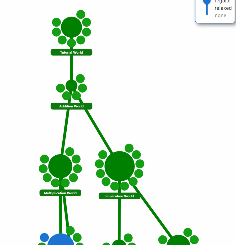
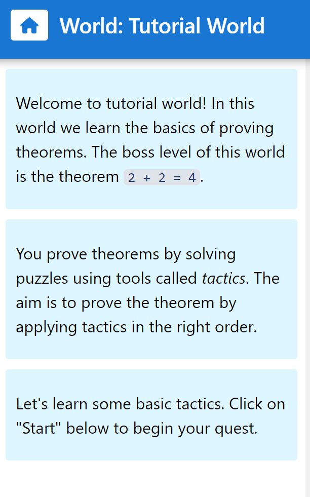
The Natural Number Game is an interactive introduction to coding with Lean. It is in many respects a great tutorial but it is also simply a fun game.
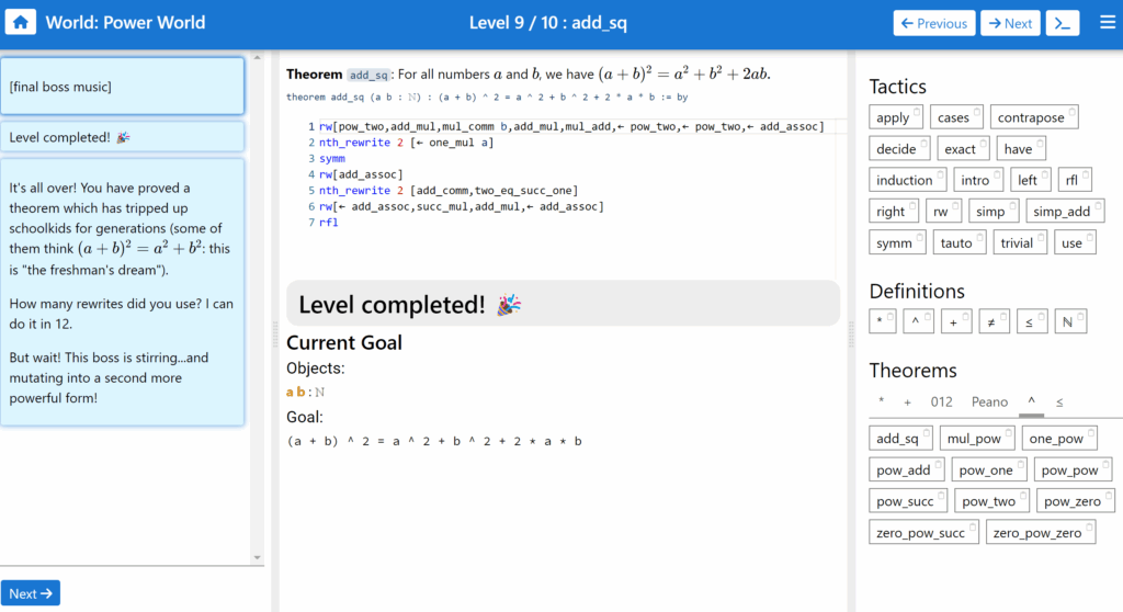
Like most games, there are multiple levels with different themes each. You start off with the goal to prove 2 + 2 = 4. All you get is a simple text interface and a sidebar with proven statements and so called tactics.
Tactics are methods or strategies one can apply in order to advance a proof. These tactics include mathematical proof techniques like induction, differentiating between cases, and turning a statement around through logical contrapose. But they also include commands like “rfl”, “tauto” or “intro”, which are special to Lean.
They stand for reflexivity, tautology, and introduction. These tactics allow the goal to be transformed, similarly to how we segment the proof of a mathematical statement into multiple steps that each need verification on their own. And this really shows the crux to understanding Lean.
While we may have an ocean of fantastic and ingenious mathematical proofs, there is not a lot of data on how their authors came up with their proofs. We may understand the logic behind them, yet we fail to understand how they are generated. And this is precisely the problem that needs to be understood when creating a language like Lean. Afterall, how would one formalize a system when the form of this system is not even clear?
This is where dependent type theory comes in! It is a theory that describes the architecture of mathematical thought. This framework is the kernel of Lean and by it we are allowed to formalize the strange way of mathematical proof writing. But more on dependent type theory later.
As you can see, the Natural Number Game already inspired some deep insight into this language. But back to the game itself.
It delivered great understanding of how Lean works and, in turn, how a mathematician’s mind might work. The idea is that, we start off with a (hopefully true) statement and our mission is to use all the knowledge and body of previous work to break apart the statement into a few facts we do know and understand. Now this procedure describes both how a mathematician works on paper and in Lean. The key difference, which appears immediately, is the chronology of the steps taken in this process. While a mathematician works forward on paper, meaning we start off with a true assumption, like all integers have an additive inverse, and then through implication or construction, we follow this assumption with a second statement that is closer to the actual statement we want to prove. In this logically rigorous manner, we step closer and closer to our original hypothesis, and in the end we say, “This statement is true because we can trace it back to a simpler, already proven fact.”
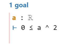
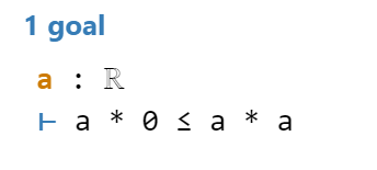
The mathematician in Lean, however, starts off with this last sentence: he already thinks, “If this statement is true, how can I simplify it to get a known fact?”. As in the game, one is presented with the statement one wants to prove. But instead of starting somewhere known, we work ourselves backwards to a true hypothesis, similarly to how one solves equations, or proves a simple algebraic inequality – by reducing the given inequality until one arrives at a given assumption. The process consists of reducing the statement through theorems and tactics. For instance, if we wanted to prove that the square of a real number is always non-negative, it would look something like this:
- \(a^2 \ge 0\)
- \(a\cdot a \ge a \cdot 0\)
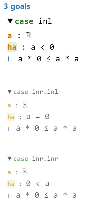
- Cases
- if \(a < 0\) then 2. implies \(a < 0\)
- if \(a = 0\) then \(0 \cdot 0 > 0 \cdot 0\)
- if \(a > 0\) then 2. implies \(a^2 \ge 0\)
Now, in all 3 cases, the last statement is always an obviously true statement and thus we successfully reduced the initial inequality and have proven the original hypothesis. In the game, this “text” would be what is displayed in the interface when writing the proof. The proof itself would then be written like this:
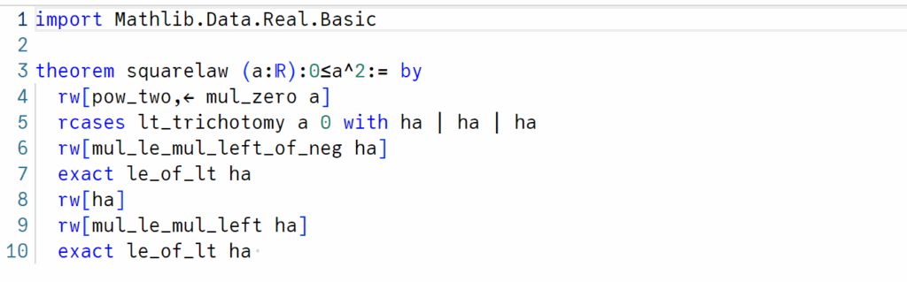
Line 3: I declare the theorem by its name, input values and statement (in that order)
Line 4: rw stands for “rewrite”. In correspondence of this code to the first proof, I transform the statement \(a^2 \ge 0\) into the statement \(a \cdot a \ge a \cdot 0\) with this first command.
Line 5: With this second command, I open up a queue for all the cases \(a < 0\), \(a = 0\), \(a > 0\) and prove them individually.
Line 6: I am now trying to prove the statement in the first case. This I do by cancelling \(a\) from both sides of the inequality under the assumption that \(a < 0\), which yiels \(a \le 0\), which is why
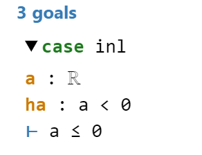
Line 7: in this line I use the exact command. This does nothing but exact our assumption, which is \(a < 0\) since we are still in the first case. With this command we conclude case 1.
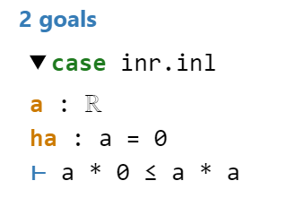
Line 8: Our goal now is to prove again \(a \cdot 0 ≤ a \cdot a\) but this in the case of \(a = 0\). This is easily proven, by simply replacing \(a\) with 0 in the inequation, which this command does.
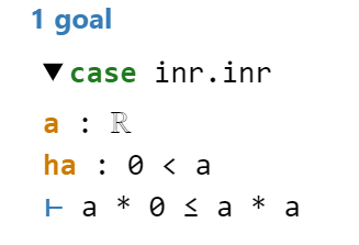
Line 9: Now for the final goal, we assume \(a > 0\). This works analogous the first case. First we cancel \(a\) from both sides and then
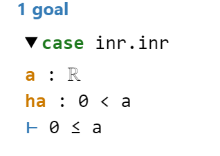
Line 10: exact our assumption and we are done.

While this code works just fine, for completeness here is the official proof from the Mathlib database:
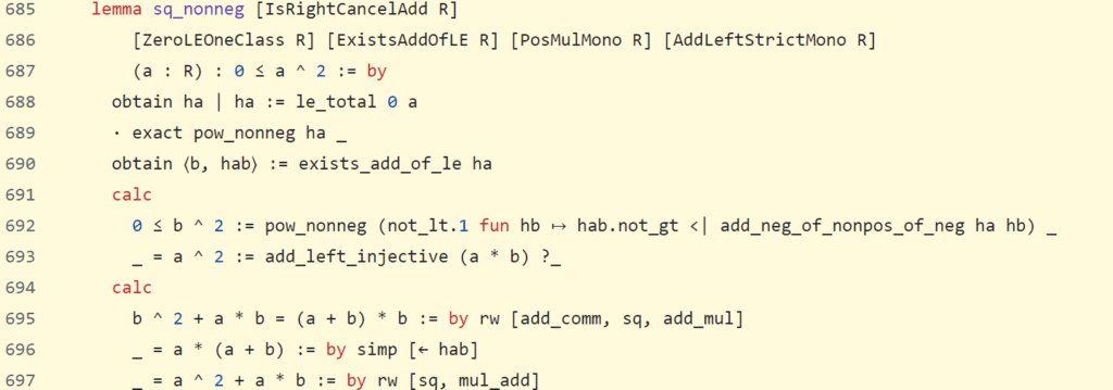
In this code you can see the command “simp” which does nothing but simplify an equation automatically. The goal of the game is to first understand how Lean operates. Thus, commands like simp are not accessible in the first part and one has to manually prove simple truths, such as the fact that additivity is commutative for all natural numbers. In actual Lean, one is, of course, equipped with most arithmetic rules and statements and can thus often use commands like “tauto” and “simplify” to prove certain equations.
Lean Introduction Guide
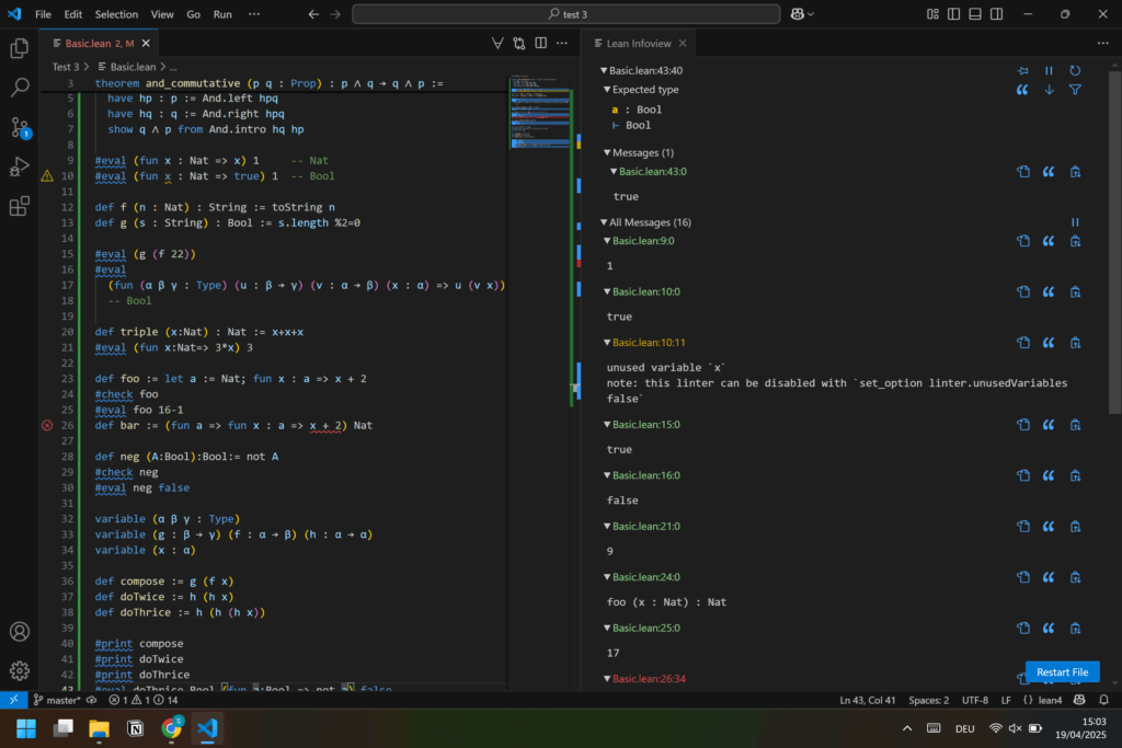
At this point of my journey, I had read a bit about Lean and played a great tutorial for it. I deemed myself a bit more braced to undertake my original task. So I downloaded and installed Lean, which is a feat in itself, downloaded the ComputableReal Repository, and opened the code I was supposed to get to know. I was hit with a wall of cryptic text again. Most of it was still gibberish but I had hope, because by now, some terminology, some syntax was known to me. I started to read but did not get far. All the gears in my head were turning and most of them in the wrong direction. I was not yet ready. So I went back to reading. This was to be my final stop before I could complete my mission.
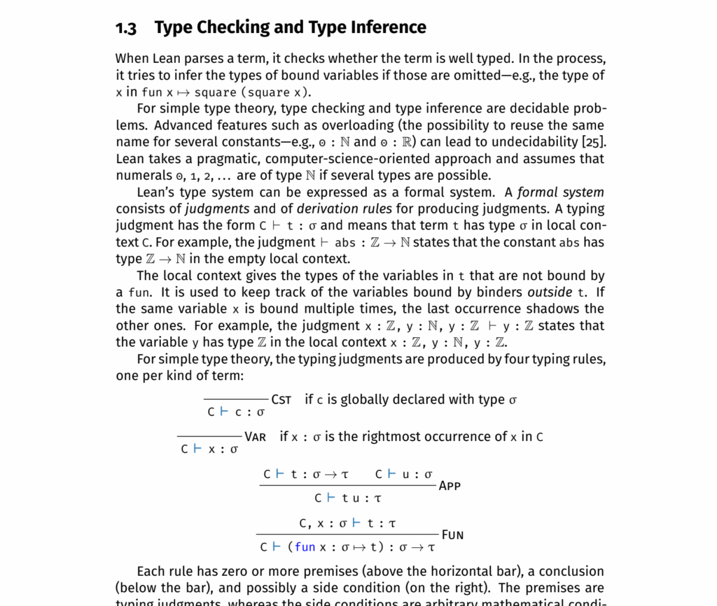
In ”The Hitchhiker’s Guide to Logical Verification”, they explicitly state that this guide would not be an introductory text to Lean but to the formalization of proofs in code. But, kindly enough, they recommended such an introductory text. So I went ahead and read that. Unambiguously, it is called “Theorem proving in Lean 4”, and it is exactly that. In the first two chapters, we are guided through the inception of how something like Lean could be built. As mentioned earlier, this is were we get to know the beautiful machinery of Lean: dependent type theory. Lean is built in this framework. Dependent type theory proposes that certain types, as we know them from other programming languages, can be dependent on the parameters they are given. First of all, what is a type and what would it mean for it to be dependent on something? A type is, roughly speaking, a class of objects, and the dependency then refers to which section of objects we want to reference in this class. For instance, the class of all lists (or arrays) is a huge set of objects containing every possible list: the boolean lists, integer lists, etc. etc. However, if we wanted to program with a list, we would specify that we want a list consisting of integers or booleans. So, you see, the type “List” would then depend on what kind of objects we want our concrete list to hold. (Another way to understand this, is as so called polymorphic functions, that assign to elements a certain type)
In this general frame, we can then define many things that we usually use in programming and mathematics, we can introduce functions and variables as types that of course vary once again on given parameters. But we can also go further and introduce mathematical notions in this type theory, namely we want propositions, logical assertions, to be a type! And this is exactly what Lean is built on. Most of the time we may think of types as a set like the real numbers, something we want to take elements from and do computations on, but in Lean we introduce propositions themselves as a type and in this way, we transform the mathematical logic into a question of correct type checking. What I mean is, imagine you have programmed a function that takes an integer and returns a double or float by dividing by two. To define this function you would have to specify both domain and target space correctly and only when this is done, is your function syntactically correct and everything performs well. Now if we replace integer and float with propositions \(p\) and \(q\) , then we would have an arrow \(p \rightarrow q\). The computer would see no difference to the first function, but we understand it as a completely different thing. This function \(p \rightarrow q\) would mean for us that the proposition \(q\) follows from the proposition \(p\). However, what would we substitute for the elementary description of our initial function? And the answer is, that we replace the definition \(x \mapsto 2\) by
\(\text{proof of } p \mapsto \text{proof of } q \text{ using } p\)
So what we do is, we write with certain operations a proof of q and at some point, we will insert somewhere a proof of p. Now what makes this function well defined, is that our proof of q can obviously only be correct, if our proof of p is correct, since the output proof builds upon the given proof (excluding for this example of course axioms and statements that are true regardless of p). In this way then, we can understand a correct proof of q as being a proposition with the correct type.
We have already seen in the Natural Number Game how a code in Lean could look, but now we can see how this code is understood by the computer! Using dependent type theory, we code a mathematical proof as nothing else but a function that given a statement constructs a different statement, and if and only if the proof is logically sound, then the function will output the correct type. So what we have done is translate a mathematical proof into a well-typed function.
An excerpt from the guide:
To some who take a constructive view of logic and mathematics, this is a faithful rendering of what it means to be a proposition: a proposition p represents a sort of data type, namely, a specification of the type of data that constitutes a proof. A proof of p is then simply an object t : p of the right type.
Understanding now how Lean works, we can finally try to read the ComputableReal code.
ComputableReal
Given that our goal is to understand an implementation of the real numbers in Lean, we might be tempted to ask, why we would even need such a thing. Although the real numbers are a self-evident part of the fabric of our lives, we calculate with them in school and don’t even think twice about a number like \(\sqrt 7\). It is nowhere near self-evident what they actually are. Every year in the introductory course Analysis, we construct the real numbers and it is first there, that we see how weird and complicated they really are. The natural numbers are so “natural” that we cannot explain them, they are axiomatically given as an inductive set, as the concept of counting itself. Only late have we figured that these numbers must have a continuous space between them, that there must be numbers in between the natural numbers. But unlike the integers and the rational numbers, how we get the real numbers, does not simply come from constructing a completion of the natural numbers under one arithmetic operation. We may take all the square roots of the rational numbers and we would still not have all real numbers!
Over the centuries we have developed many ways of constructing \(\mathbb R\), one more complicated than the other (https://en.wikipedia.org/wiki/Construction_of_the_real_numbers). It is this difficulty of construction that make the real numbers so hard to computationally implement. One general approach is to just approximate them with rational numbers. For instance, every real number can be represented as the supremum of some set of rational numbers, practically we could thus construct a convergent series of rational numbers that we would cut off at some point if its distance from the real number that we are trying to get is negligable. And this is somewhat the approach of encoding the real numbers in a computable way, the way it was done in this Repository.
Now in standard Lean there is already a version of the real numbers, that one can use. This version however is logically constructed in the same way as described above: we represent a real number with a sequence of rational numbers that converges to it. Since there are multiple such sequences that converge to the same value, we must identify these sequences with each other. And so a real number in Lean is actually a “set” of many, many so called Cauchy sequences that all approach the same target. This bizarre concept would defy anyone’s ordinary idea of a number. How would one even do any calculations with such an object? And this is where the standard implementation of Rand the ComputableReal Repository diverge.
The standard implementation keeps the real numbers as these logically constructed objects and infers all the properties from this construction. So, when we come face to face with a real number we may use these properties and theorems to do our proving but we have no actual numerical value attached to what we are working with. We may prove something like \(1 \le \sqrt 2\) by hand with the standard implementation (by squaring both sites for instance), but Lean on its own has no way of actually knowing, since there is no actual value for \(\sqrt 2\), only a description and some properties. In ComputableReal however, just as the name suggest, we actually have a numerical value with which we can do calculations. We arrive at a value as described above, again with Cauchy-Sequences but this time we simply demand that these sequences can be algorithmically computed.
In this way we can understand the ComputableReal numbers not so much as a different implementation of the reals, but as a suitable subset of \(\mathbb R\) in Lean, that we can equip with more arithmetic structure.
In this manner we can build a function “native_decide” that can prove an inequality like \(1 ≤ \sqrt 2\) simply by actually comparing the approximating sequences of \(\sqrt 2\) with \(1\). Since almost every member of a Cauchy Sequence that converges to \(\sqrt 2\) is bigger than \(1\), our comparison function does not take long to compute.
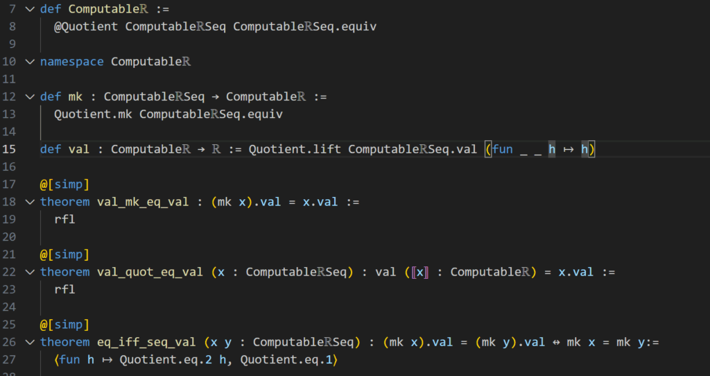
Getting more technical, in these first lines of code we can see the declaration of the Computable\(\mathbb R\)numbers as quotient of Computable\(\mathbb R\)Seq Sequences. The equivalence relation here is that two sequences are identified, if they converge to the same value.
This equivalence relation is defined by this code:
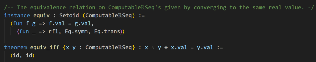
Here fun f g => f .val = g.val defines two Cauchy Sequences \(f, g\) to be equal, if their limits f.val and g.val are equal. The second part of this definition is a proof that this defines an equivalence relation.
To understand how the limit of such a Cauchy-sequence is determined, we need to understand, that the sequences in Computable\(\mathbb R\)Seq are objects consisting of two actual sequences, one sequence of successive lower bounds and one for upper bounds of the value that is approximated. In this way we can approach the real number in a precise and computationally intelligent way. Having upper and lower bounds is the key that enables us to make statements about the real numbers even if we can’t fully compute them. Again the example \(1 ≤ \sqrt 2\) shows exactly this. The lower bound sequence of \(\sqrt 2\) is always bigger then the upper bound sequence of \(1\) and thus we can derive a proof of this inequality even without the actual value of \(\sqrt 2\). So the entire main engine of this implementation is built around this approximation through upper and lower bounds.
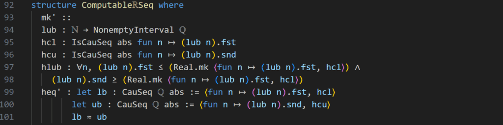
The question yet remains, how is this programmed? In the code above the structure of these computable\(\mathbb R\)Seq Sequences is given. (We have not looked at what actually constitutes a structure in Lean but for our purposes here it is sufficient to think of this structure as a declaration of a type). To capture the thinking explicated above, we interpret a sequence as a function from the natural numbers, this we can see with the lub declaration. lub is supposed to be our sequence of lower and upper bounds, so each item in our sequence is a pair of two numbers. (This coupling, we actually understand as an interval to make use of the library of interval arithmetic but this text will not go into detail about that). Now our intent was to encode two Cauchy sequences of upper and lower bounds that both converge to the same real number. This is simply done by asserting that the first component of our pair sequence \(l_n\) is actually a Cauchy sequence, the name of this assertion is hcl which is an acronym for hypothesis-Cauchy-lowersequence. Analogously, we treat the upper component sequence \(u_n\) with hcu. Then the assertion hlub demands that the two sequences are actually sequences of upper and lower bounds of the same number. You can see this by understanding that “Real.mk ⟨fun n ↦ (lub n).fst, hcl⟩” is simply refering to the limit of the lower bound Cauchy sequence, so replace this line with \(l := \lim_{n\rightarrow\infty} l_n\). That way we can see hlub in mathematical notation as \(l_n \le l \land u_n \ge l\). And finally the command heq′ is a proof that both of these sequences that we have now defined to be upper and lower bound Cauchy-sequences of the same number, actually converge to the same number.
A computable real number is thus a class of upper and lower boundary rational Cauchy-sequences, that all converge to the same limit. What makes this computable is that the Cauchy-Sequences are successive lower and upper bounds of the number they converge to, unlike the Cauchy-Sequences that are used to define the numbers in type \(\mathbb R\)!
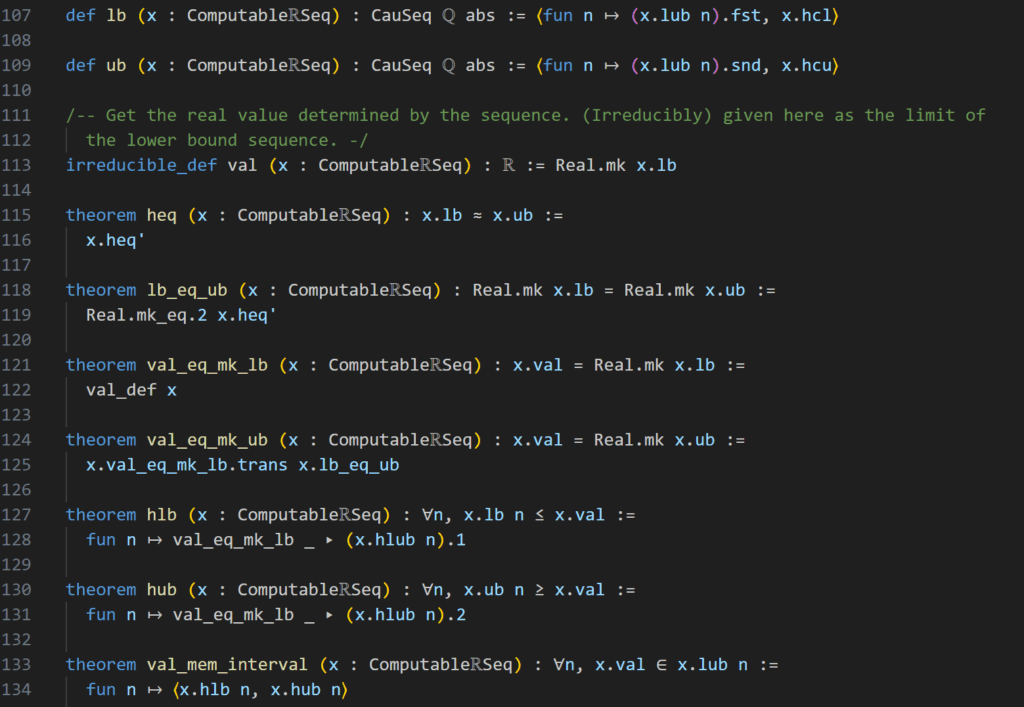
Now getting back to our first excerpt (Fig. 10), we see in line 12 a definition of the canonical projection from Computable\(\mathbb R\)Seq to its quotient Computable\(\mathbb R\) denoted by \(m_k\), so x.mk denotes a (computable) real number, while x may be a sequence. Next we have another important function val, this is an imbedding of the computable real numbers we have just constructed into the standard real numbers, so that (x.mk).val denotes a number of type \(\mathbb R\) in Lean. As mentioned above, we can think of the Computable real numbers as a subset of real numbers, precisely all the real numbers, that have lower and upper bound Cauchy-sequences. These definitions are important since we want (need) to build the machinery of this repository in Computable\(\mathbb R\)Seq but want the application to be usable in \(\mathbb R\).
What follows is a list of simplifying theorems (continuing way after this excerpt). These lay the notions for how Lean is supposed to understand all of this. For instance, the first of these theorems states nothing else but that the real number value of an equivalence class x.mk is nothing else but the limit of the Cauchy-Sequence x. This as the name implies simplifies things, such that instead of doing our proof on an equivalence class, we can use the theorems from Computable\(\mathbb R\)Seq directly on any representative of this class.
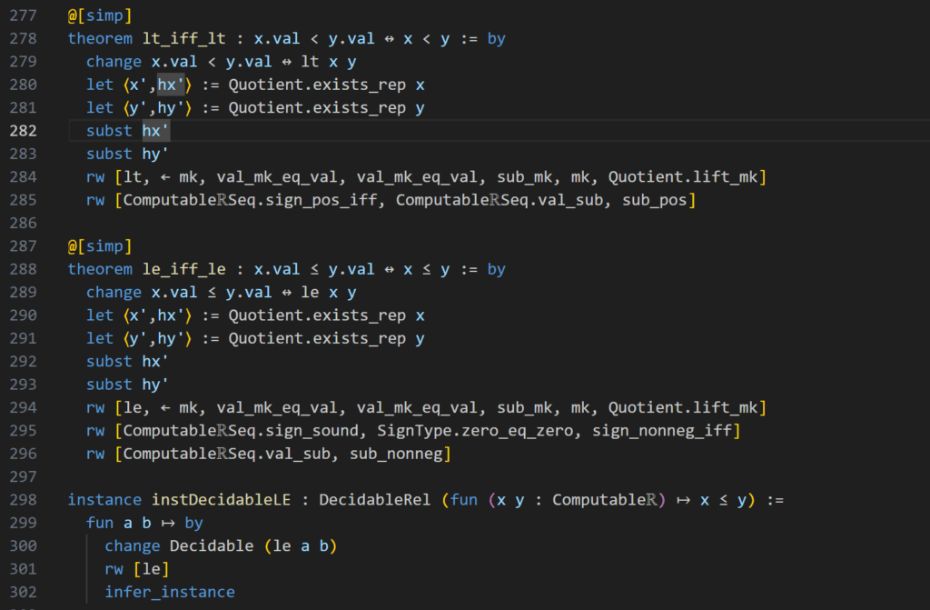
In this manner, step by step, the code develops properties and tools for this new structure Computable\(\mathbb R\), until there is enough machinery to construct a function like “native_decide” as above.
However, the biggest flaw of this approach through upper and lower bound sequences is around zero. When we have a Cauchy sequence with limit zero, then its upper bounds must be greater than zero and its lower bounds lesser and this difference in signs breaks down this entire awesome engine. This happens simply because this code continues to approximate these bounds with more and more precision until both of them have the same sign. But with upper bounds that are always above zero and lower bounds that are always below zero, this approximation runs on ad infinitum! So we are absolutely helpless when we are faced with anything of the type \(\pi − \pi = 0\). Of course this makes all equations with real numbers impossible to prove with “native_decide”.
While working with equations may be the next step, we are now equipped with the ability to do inequations! Almost any inequation with irrational numbers is now approachable with this new implementation. So, even though, there is still room to grow, we have reached a great milestone in formalizing arithmetic with real numbers. Something like \(1 < π\) is now obvious in Lean!
Conclusion
In conclusion, while this implementation is a great milestone that provides Lean with a new powerful set of tools, it is by far fully fledged out. We now have a powerful new tool for inequalities of real numbers. Making arithmetic with all numbers greatly more accessible, however, the mere fact that an equation of the type \(\sqrt 5 = \sqrt 5\) is still unprovable by this method, shows the great limit of this current implementation.
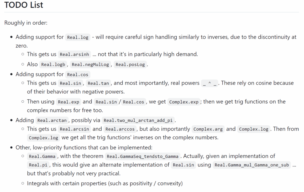
The authors of this code although are by far not finished. And a look on github reveals a list of their next goals.
Links
- https://github.com/Timeroot/ComputableReal
- https://github.com/leanprover-community/tutorials4
- https://github.com/leanprover-community/mathlib4
- https://discourse.julialang.org/t/scilean-language-interactive-and-mathematicaly-sound-code-transformations/81101
- https://adam.math.hhu.de/#/g/leanprover-community/nng4
- https://leanprover.github.io/theorem_proving_in_lean4/
- https://lean-lang.org/functional_programming_in_lean/introduction.html
- https://lean-lang.org/lean4/doc/quickstart.html
- https://lean-lang.org/doc/reference/latest/The-Type-System/Quotients/?utm_source=chatgpt.com
- https://en.wikipedia.org/wiki/Construction_of_the_real_numbers#
- https://leanprover-community.github.io/mathlib4_docs/Mathlib/Data/Real/Basic.html
- https://www.ma.imperial.ac.uk/~buzzard/xena/formalising-mathematics-2022/Part_A/section02reals/reals.html