Written by Aaron Osburg
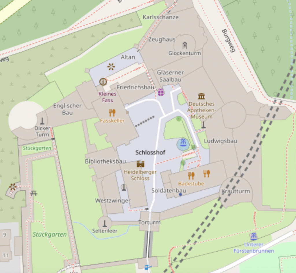
Imagine you are planning your birthday party which will take place in Heidelberg Castle. You have a lot of friends, so you are not quite sure if the inner courtyard of the castle provides enough space for all your guests, the buffet, and the live band. Unfortunately, you are visiting your grandmother these days and she does not have a computer that you could use to calculate the area of the courtyard and all you have is a printout of the map you can see below. You notice that it has such an irregular shape that your high school math skills could not help you either. Damn it, this is going to be the worst birthday party ever!
Later this day you see an old and dusty case on the shelf that you have never noticed before. You open the case and inside you find this device.
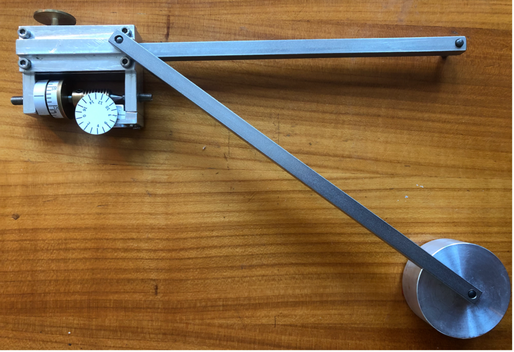
You have never seen something like this before, so you ask your grandmother what it can be used for. She explains the device you hold in your hands is called “polar planimeter” and can be used to measure the area of a plane surface by tracing out its boundary. It consists of a pole (lower right corner) connected to a rod, the so-called pole arm. On the other end of the pole arm there is a hinge connection to a second rod, the tracer arm. Additionally, a tracer (upper right corner) and a measurement wheel (upper left corner) are connected to the tracer arm. To measure the area of a surface you place the pole outside the surface and the tracer on the boundary of the surface. After setting the measurement wheel to zero and carefully tracing out the boundary of the surface you can read the area off the scale on the measurement wheel.
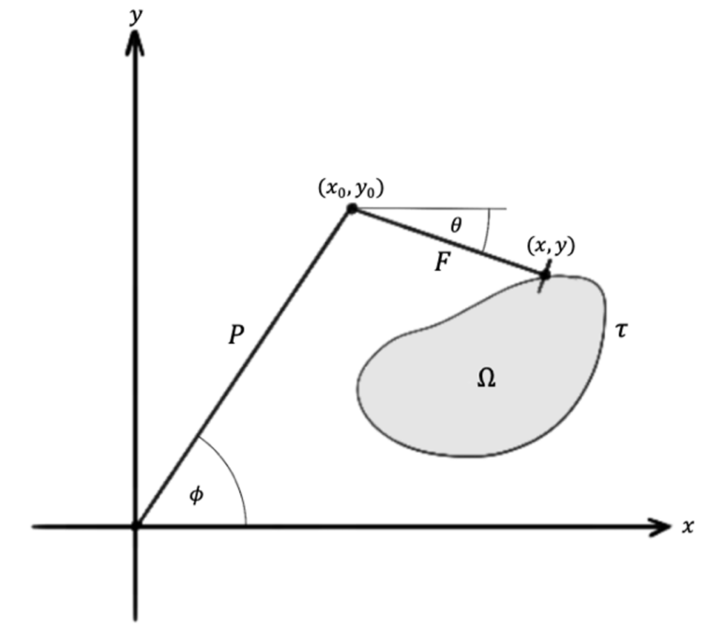
Mathematically, the polar planimeter is an application of Green’s Theorem. The measurement wheel is aligned in such a way that the net rolled distance \(\mathcal{PM}(\tau)\) is
\( \mathcal{PM}(\tau) = \int_{\tau} – \frac{y – y_0}{F} \: dx + \frac{x-x_0}{F} \: dy\, , \)
after the tracer has moved along a curve \( \tau \) in the situation of figure 3. For simplicity, we assume that the measurement wheel is at the same position as the tracer.
In case of a domain with piecewise smooth boundary in \( \mathbb{R}^2 \) with boundary curve \( \tau \) it follows from Green’s Theorem that
\( \mathcal{PM}(\tau) = \frac{1}{F} \int_{\Omega} dx \wedge dy\, . \)
The proportionality factor \(1/F \) can be integrated into the scale on the measurement wheel so that it shows the correct value for the area after the measurement.
This is exactly what you needed! A quick measurement with your grandmother’s polar planimeter shows that the courtyard has an area of \(3668 \, \text{m}^2 \), which is precisely the amount of space you need for your party!
You have even more luck: there are two types of planimeters exhibited at the HEGL Lab. If you want to learn more about planimeters and the mathematics behind them or just want to play around with them, feel free to visit us!
The image credits of figures 2 and 3 go to the blog post author.