Written by Ricardo Waibel in collaboration with Donald Youmans
Topology and geometry are important concepts in mathematics and physics. Especially in theories like general relativity they have a direct impact, as the spacetime description of a system is already quite geometrical.
To highlight the difference between the two concepts, let’s look at a simple two-dimensional disc first. An interactive visualization of it can be found here, with several operations you can perform. For example, you can push and stretch the centre of the sphere up and down, or perform several twists.
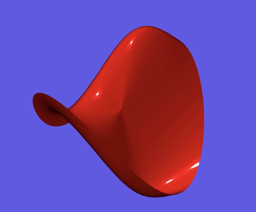
These operations can be performed in a smooth and continuous way; we would say, that the geometry of the object is changed, but not its topology. This can be seen by trying to contract the disc continuously to a point. It works always for the disc, even when deformed first.
If we punch a hole in the middle of the disc instead, we have performed a non-continuous operation. This turns the disc into an annulus:
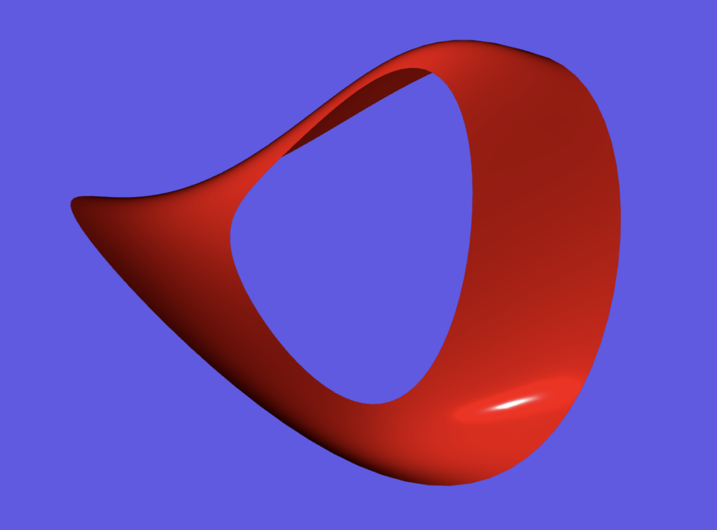
We can perform the twists and deformations again, but if we try to retract it, a small circle will always be left over. This circle cannot be retracted to a point in a continuous manner, which shows that topologically, the disc and the annulus are different.
The lesson is basically that expanding, stretching, twisting, i.e., continuous deformations, do not change the topology of a space, but cutting or punching a hole into it will do so. In that manner, the topology of an object represents more the underlying structure of a space (which in two dimensions can be reduced to the question of how many holes exist) or in other words, a more global perspective on an object. Geometry on the other hand is a more subtle description of how much a space twists and curves, a local perspective on such properties like distance measurements and curvature.
A physical example that showcases geometry and topology is a wormhole. There are different examples of wormholes, here we have chosen the so-called Ellis wormhole, named after Homer G. Ellis, which was also independently described by Kirill A. Bronnikov at the same time [1]. The spacetime can be described by the following metric (a way of measuring distances in the object)
\(\text{d} s^2 = -\text{d} t^2 + \text{d} \rho^2 + (\rho^2 + a^2)\, \text{d} \Omega^2\ ,\)
with the parameter \(a\) describing the width of the central hole, \(t\) representing time, \(\rho\) a coordinate, and \(\text{d} \Omega\) the angular part of the volume element, which can be expressed with two further coordinates \(\theta\), \(\phi\) as
\( \text{d} \Omega^2 = \text{d} \theta^2 + (\sin(\theta))^2\text{d} \phi^2\ .\)
As a solution to the equations of general relativity, this represents a four-dimensional space. To find a way of displaying this as a two-dimensional object in a three-dimensional surrounding space, we need to fix two coordinates: we take the equatorial cross-section, which is given by \(t=0\), \(\theta=\frac{\pi}{2}\). This then has the special metric
\( \text{d} s^2 = \text{d}\rho^2 + (\rho^2 + a^2)\, \text{d} \phi^2\ , \)
where the coordinate \(\phi\) describes the position on a horizontal circle cross-section, and \(\rho\) the distance from the central circle of the throat. To find a parametric description from this, a bit more work has to be invested. First, we change the coordinates slightly, then we compare them to a known coordinate description. Change to \(r^2 = \rho^2 + a^2\), which gives
\( \text{d} s^2 = \frac{\text{d} r^2}{f(r)} + r^2 \text{d} \phi^2\ , \)
with \(f(r) = 1 – \frac{a^2}{r^2}\).
Cylindrical coordinates \((r,\phi,z)\) should be suited to this problem, and in three-dimensional space they have the description
\( \text{d} s_\text{cyl.}^2 = \text{d} z^2 + \text{d} r^2 + r^2 \text{d} \phi^2\ . \)
Now viewing the coordinate \(z\) as dependent on \(r\), i.e., \(z=z(r)\), we can write this as
\( \text{d} s_\text{cyl.}^2 = (1+z'(r))\,\text{d} r^2 + r^2 \text{d} \phi^2\ . \)
By simple comparison, we derive the following differential equation
\( 1 + z'(r) = \frac{1}{f(r)} = \frac{r^2}{r^2 – a^2}\ , \)
which can be solved by direct integration. The result is
\( z(r) = a \cdot \cosh\left(\frac{r}{a}\right) \ . \)
This can then be visualized, which can be found here.
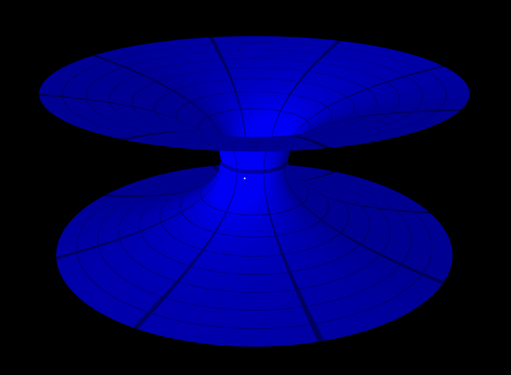
The view on the blue wormhole is a view from outside the spacetime, i.e., an observer in that spacetime would see it very differently. Grid lines on the object show how deformed it is. The parameter \(a\) of the wormhole can be changed, as well as some simple geodesics can be displayed (geodesics are the shortest paths connecting two points, in a general spacetime).
Wormholes represent substantial changes to a spacetime (topological changes), and this can be seen when this wormhole connects two parts of a spacetime that would have previously been unconnected. The following is a 3D print produced at the Lab, which shows just such a scenario (you can read more about such things in [2]):
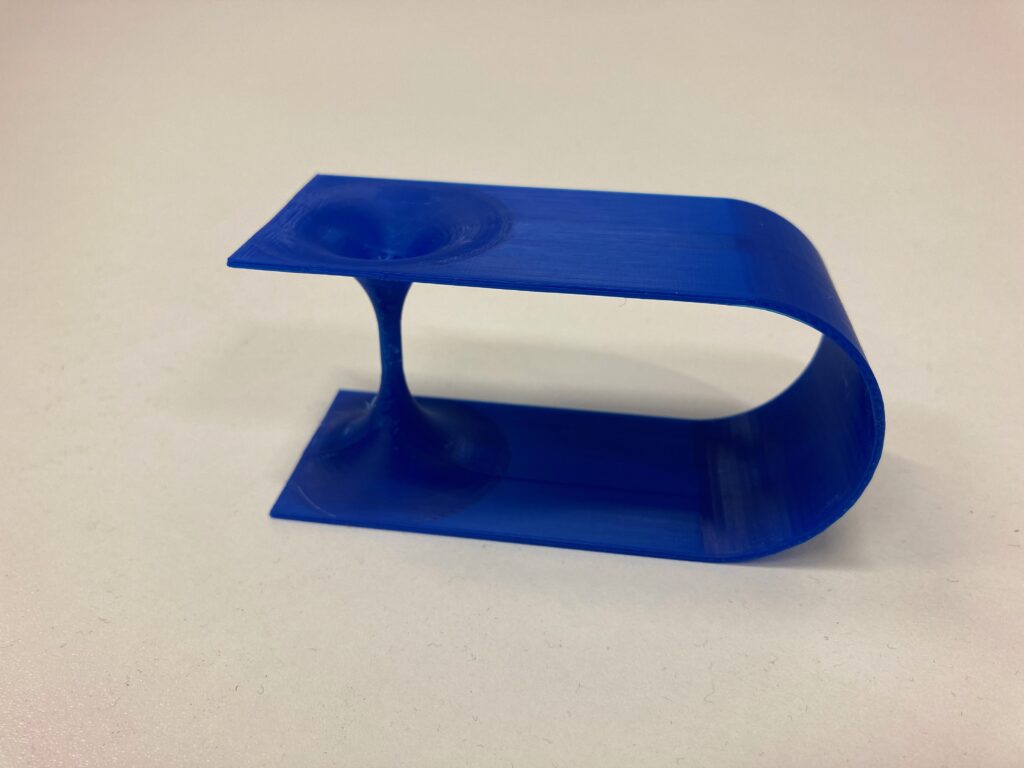
Imagine a person on the top, close to the wormhole. Going to the bottom part of the object would usually only be possible the long way around, via the right part of the bridge. But now that the wormhole is in there, a shorter path exists (this is why wormholes are connected to time-travel and faster-than-light space travel (if you could create one)).
Have fun playing around with the visualizations or drop by the lab if you want to see the 3D print. If you want to know more about how a wormhole looks like to an observer living inside the spacetime, check out [3].
References: