Continuous Cellular Automata

In a Cellular Automata, we simulate a grid of cells. For each cell, we can calculate its upcoming state based on its previous state.

A very famous example of such a system is Conway’s Game of Life. In the Game of Life, each cell can be either dead or alive. We can determine whether a cell will be alive in the next step using a very simple set of rules:

1. Count the number of alive neighbors of the cell
2. If the cell is alive and the number of neighbors is either two or three, then the cell stays alive, otherwise, it dies
3. If the cell is dead and the number of neighbors is precisely three, then the cell turns alive again, otherwise, it stays dead

Using these rules we can already achieve quite complex patterns, you can find a simulation of the Game of Life already containing a pattern below, feel free to play around with it and maybe discover other interesting patterns:

Lenia

Lenia is a Cellular Automata that has been derived from the Game of Life. Unlike the Game of Life, it is a continuous Cellular Automata, which means that the states of cells, as well as time and space, are continuous.

Continuous States: To make states continuous, a cell can no longer just be alive or dead like in the Game of Life. Instead, its state is on the interval \([0,1]\), where 0 would have previously represented a dead cell and 1 an alive cell. To have cells with states that are not just 0 or 1 we need continuous time steps, which are explained in the next paragraph.

Continuous Time: First we introduce a growth function, that, based on the current state of the cells, returns the amount by which the state of a cell changes. In the case of the Game of Life, this would either be \(-1\) if the cell dies, \(0\) in case the state doesn’t change, and \(1\) if it comes back to life. In the case of Lenia the growth function is \(\mathrm{growth}(x) = 2\exp\left[-\left({x-\mu \over \sigma}\right)^2 / 2\right] – 1\), where \(x\) is the sum of the weighted neighbors as explained in the paragraph Continuous Space. Instead of just outputting -1, 0, or 1 this function returns values between -1 and 1.
Next, we select an update frequency \(F\) and scale the result of the growth function by \(1/F\) before applying them to the current state of the cell. So the next state is the sum of the current state plus the scaled value of the growth function. For \(F \rightarrow \infty\), we achieve continuous time steps, since the amount of time each step represents converges to 0.

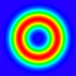
Continuous Space: Previously, we only used the direct neighbors of a cell to determine its next state. Instead, we now consider every cell within a square centered around the current cell. This square has size \(2R + 1\), for \(R \rightarrow \infty\), the space becomes continuous. We assign each neighbor within the square a weight that determines its importance in the updated state. These weights are represented using a kernel. In the case of Lenia this kernel has a donut-like shape:

Combining all of these changes leads to Lenia, you can see a simulation of Lenia already containing a moving creature called Orbium below, feel free to play around with it to maybe find your own creatures:

Particle Lenia

When playing around with Lenia, you might have noticed that there are many states where the mass keeps increasing.

Particle Lenia fixes this by simulating individual particles \(p_i\) instead of cells on a grid. By doing so, the amount of mass is fixed to the number of particles that are being simulated.

To do so, a field \(U(x) = \sum_{i}K(||x-p_i||)\) is computed, where \(x\) is the position and \(K\) a kernel similar to the one in Lenia. Based on the field \(U\) the growth of an area is calculated using another Kernel. A high growth value attracts particles, and a low value repulses them.

To prevent the clumping of particles, a repulsion force between individual particles is introduced. The sum of the growth force and repulsion force is the force acting on the individual particle.

Below, you can find a simulation of Particle Lenia:

Implementation

Lenia

During my Praktikum I implemented the Game of Life and Lenia using OpenGL to allow running them on the GPU (you can find the implementation here).

To improve performance, I explored how to compute Lenia using Fast Fourier Transformation and then implemented the Cooley-Tukey FFT algorithm as a compute shader and used it to perform Lenia steps. This changes the performance of the trivial implementation from \(O(n, R) = n^2R^2\) to \(O(n,R) = n^2\log(n)\), where \(n\) is the number of columns/rows in the grid and \(R\) the size of the kernel. This should in theory improve the performance for large values of \(R\).

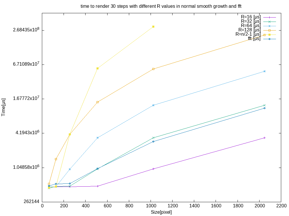
As shown by the above benchmark, you can start seeing performance increases in the FFT implementation compared to the trivial one for \(R\ge32\).

In addition to comparing the FFT implementation to the trivial one, I also compared a Python implementation using FFT to the OpenGL one.

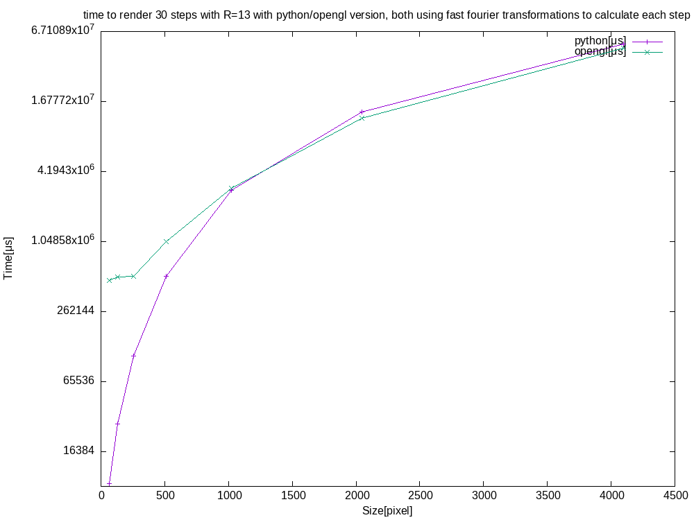
For big input grids, both versions perform quite similarly, even though the Python version is CPU bound. This is most likely due to how optimized the FFT algorithm in NumPy is compared to the Cooley-Tukey algorithm used in the OpenGL version.

Using the knowledge gained from implementing Lenia for the GPU, I also implemented it in Javascript using p5.js for this blog. The version running at the beginning of the blog uses FFT, you can find the FFT version here and the unoptimized version here. Comparing them side by side, it should be easy to spot the performance differences.

Particle Lenia

I implemented Particle Lenia using OpenGL (you can find the implementation here). The repository contains a working 2D version of Particle Lenia, that visualizes the different fields that are acting on the particles and allows the user to freely move the position of the camera as well as to add and remove particles. Below, you can see a short clip of the GUI:

It also contains some first steps towards a simulation of 3D particle Lenia.

In an attempt to improve the performance of Particle Lenia I implemented it on the CPU (the implementation can be found here) and instead of calculating the force each particle applies to the other, only did so for particles within a certain range. The range is determined by the distance after which the maximum error of all possible particles outside the range on the position of a particle after one step is lower than a given error threshold. To allow for easy access to all particles within a certain area, all particles are stored in buckets, with each bucket belonging to a part of the area.

Assuming that all particles remain evenly distributed across the 2D plane, this should lead to a near-linear runtime.

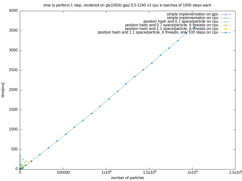
To further improve performance, I also added a multithreaded version. Below, you can find a performance comparison between the GPU version/ and the CPU version.

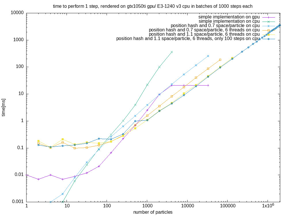
For big inputs, the CPU versions perform near linear, below you can find a benchmark where the last version ran for even more particles.

The demo implementation in this blog post also uses the technique described above, you can find all demo implementations here.