Written by Helen Freytag and Ronya Ramrath.
Inspired by Escher’s experimentation with hyperbolic art (and driven by the tempting availability of 3D printers in the clearly very well-funded experimental geometry lab), this project was concerned with extrapolating and printing the hyperbolic tessellations that form the basis of Escher’s Circle Limit series.
M. C. Escher, who had always shown a proclivity for patterns, was first introduced to hyperbolic geometry upon meeting the mathematician H. S. M. Coxeter at an exhibition of his work funded by the International Congress of Mathematicians in 1954. In their subsequent correspondence, Coxeter sent Escher a copy of his paper Crystal Symmetry and its Generalisations which contained the following image:
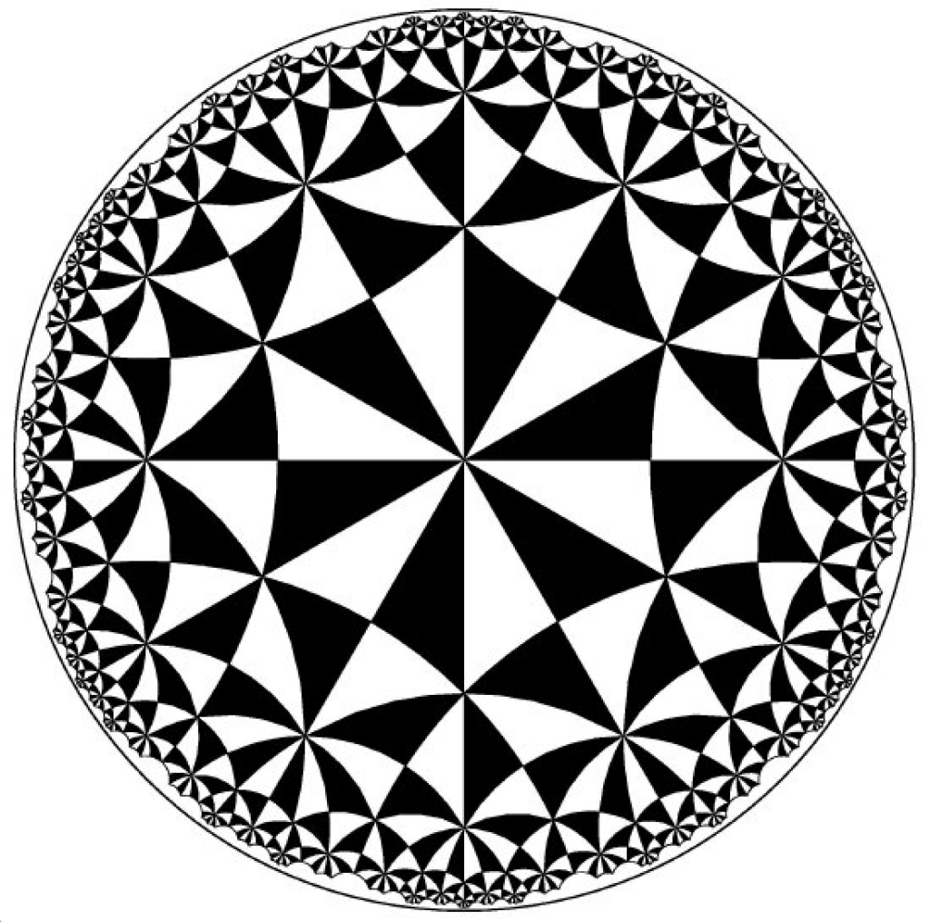
Escher was thrilled:
Though the text of your article […] is much too learned for a simple, self-made plane pattern-man like me, some of the text-illustrations […] gave me quite a shock. Since a long time I am interested in patterns with ‘motives’ getting smaller and smaller till they reach the limit of infinite smallness. The question is relatively simple if the limit is a point in the centre of a pattern. Also a line-limit is not new to me, but I was never able to make a pattern in which each ‘blot’ is getting smaller gradually from a centre towards the outside circle-limit, as shows your Figure 7.
Coxeter, 1979
Though he struggled with working out the detailed geometric construction, he created a first woodcut, Circle Limit I, on the basis of Coxeter’s figure. Although considered quite accomplished, Escher regarded it as displaying a number of shortcomings:
Not only the shape of the fish, still hardly developed from rectilinear abstractions into rudimentary animals, but also their arrangement and relative position, leave much to be desired. […] There is no continuity, no ‘traffic flow’, no unity of colour in each row.
Coxeter, 1979
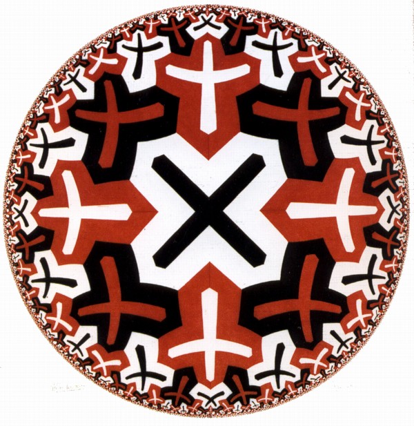
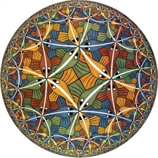
He sent a copy to Coxeter with his next letter, asking for a simple method for constructing such patterns. Based on the remarks he received in return, he then went on to explore these ideas in detail and created the following three woodcuts:

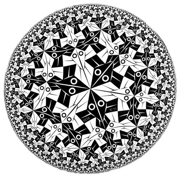
He was particularly proud of Circle Limit III, in which he considered most of the shortcomings of his first attempt eliminated:
We now have only ‘through traffic’ series: all the fish of the same series have the same colour and swim after each other, head to tail, along a circular arc from edge to edge. The nearer they get to the centre, the larger they become.
Coxeter, 1979
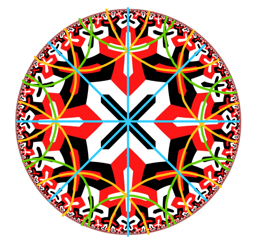
The task we set ourselves now was to extrapolate the hyperbolic tessellations that present the ‘framework’, so to speak, of Escher’s Circle Limits, and print these as 3D models. A simple sketch following the geodesics hinted at by his patterns made finding the tessellations quite easy – more difficult was the step of actually implementing these in Python. We ended up working with a code template available as part of the hyperbolic package, and though the unfortunate lack of comments made adjusting the outputs rather difficult, we managed to satisfactorily approximate each of the tilings once we figured out how the code worked.
A commented copy of our code is available on Github, but the basic idea is this:
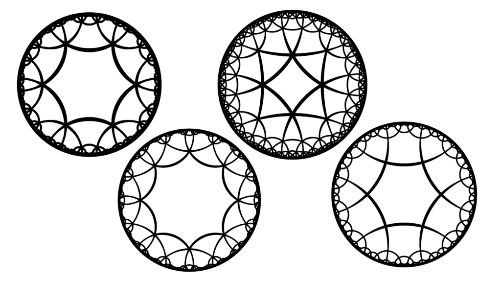
The code produces mainly quasi-regular tessellations of the type \(\{p_1,p_2,q\}\)(which is not to be confused with the Schwarz triangle tiling \(\{p,q,r\}\)!), which feature an alternating tessellation of two polygons. The number of edges of the primary polygon (the one located in the centre) is given by the value \(p_1\), the number of edges of the secondary polygon (with which the primary polygon alternates) is given by \(p_2\). Finally, the value \(q\) determines how many of each of these polygons meet at each vertex of the tessellation. A necessary condition for a configuration to work is that \(\frac{1}{p_1} + \frac{1}{p_2} + \frac{1}{q} < 1\), which can be shown as follows:
At each vertex, \(q\) \(p_1\)-polygons and \(q\) \(p_2\)-polygons meet, with respective interior angles \(t_1\) and \(t_2\), thus \(q(t_1+t_2)=2\pi\). Furthermore, since this is the hyperbolic plane, each interior angle must be less than its Euclidean counterpart, therefore \(t_1 < (p_1-2)\frac{\pi}{p_1}\) and \(t_2 < (p_2-2)\frac{\pi}{p_2}\). Taking these conditions together, we get:
\(\quad \ q((p_1-2)\frac{\pi}{p_1} + (p_2-2)\frac{\pi}{p_2}) > 2\pi \\ \Rightarrow \frac{(p_1-2)}{p_1} + \frac{(p_2-2)}{p_2} > \frac{2}{q} \\ \Rightarrow 1 – \frac{2}{p_1} + 1 – \frac{2}{p_2} > \frac{2}{q} \\ \Rightarrow 1 > \frac{1}{p_1} + \frac{1}{p_2} + \frac{1}{q} \)
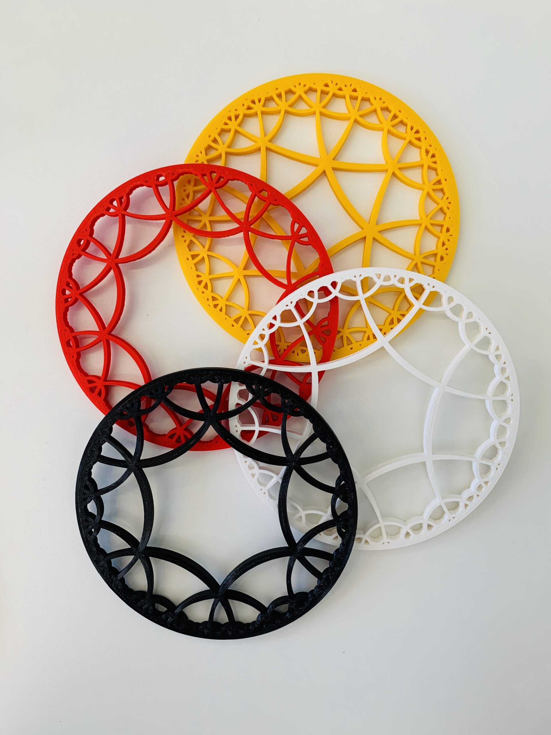
We played around with the code for a while to produce satisfactory renditions of each tiling suited for the scale we were aiming at and within the capabilities of the 3D printer. We also found we had to retrace the hyperbolic lines with Euclidean ones to ensure a minimum thickness where the former became too thin along the edges, while trying to maintain the hyperbolic contrast of thick centre lines vs thinner outer ones. We then exported the files as high-definition pngs and extrapolated the edges as dfx files using Inkscape. Assisted by Mathias Häberle, we used Solidworks to create an extrusion and finally print the images as 3D models. These are now available to view in the lab and on thingiverse.

References:
- Coxeter, H. S. M., 1979, “The Non-Euclidean Symmetry of Escher’s Picture ‘Circle Limit III’”, Leonardo, vol. 12, no. 1, pp. 19-25.
- Dunham, D., (2003), “A Tale Both Shocking and Hyperbolic”, Math Horizons, vol. 10, no. 4, pp. 22–26.
- Joyce, D. E., (1998), Hyperbolic Tessellations, available at: http://aleph0.clarku.edu/~djoyce/poincare/poincare.html
Image Sources
- Coxeter’s Tessellation: Coxeter, H. S. M., 1979, “The Non-Euclidean Symmetry of Escher’s Picture ‘Circle Limit III’”, Leonardo, vol. 12, no. 1, p. 19.
- Circle Limit I: https://www.wikiart.org/en/m-c-escher/circle-limit-i
- Circle Limit II: https://mathstat.slu.edu/escher/index.php/File:Circle-limit-II.jpg
- Circle Limit III: https://en.wikipedia.org/wiki/File:Escher_Circle_Limit_III.jpg
- Circle Limit IV: https://mathstat.slu.edu/escher/index.php/File:Circle-limit-IV.jpg
(Note: All images were used in accordance with the respective source’s fair use policy.)