Written by Alassane Diagne and Ayşegül Peközsoy
Möbius transformations are functions of the form \(T\colon \mathbb{C}\rightarrow\mathbb{C},\ T(z) = \frac{az+b}{cz+d}\) with \(a\), \(b\), \(c\), \(d\) complex numbers. We often associate the mapping \(T\) with the matrix \(T=\begin{pmatrix}a&b\\ c&d\end{pmatrix}\).
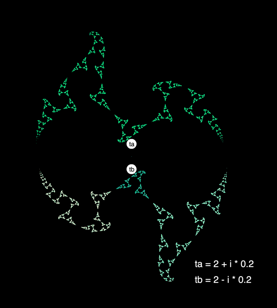
If you look at the bottom of the page, you can see some pictures we created in our project with an algorithm that is heavily based on Möbius transformations. So how do we get these pretty pictures out of these seemingly boring functions? To answer that question, we first have to give a few fundamental definitions.
First of all, we are only going to look at a specific class of Möbius transformations: loxodromic transformations. A Möbius transformation \(T\) is called loxodromic if \(\text{trace}(T)^2 \in \mathbb{C} \setminus [0,4] \). The reason why we look at these transformations specifically is that they have two fixed points. A point \(p\in\mathbb{C}\) is a fixed point of the Möbius transformation \(T\) if \(T(p)=p\). We call a fixed point \(p\) attracting if the points close to \(p\) get mapped closer to \(p\) by \(T\). We also write \(\text{Fix}^+(T)\) for the attracting fixed point of \(T\). Similarly, we call a fixed point \(p\) repelling if the points close to \(p\) get mapped further away from \(p\) by \(T\). We also write \(\text{Fix}^-(T)\) for the repelling fixed point of \(T\). Loxodromic Möbius transformations have each one attracting and one repelling fixed point.
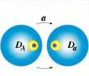
Next, we have to learn what Schottky disks are. Möbius transformations have the interesting property that they map circles to circles. For a loxodromic Möbius transformation \(a\) and its inverse \(A\) we can find two disks \(D_a\) and \(D_A\) such that they fulfil five properties:
- The disks \(D_a\)and \(D_A\) do not overlap.
- The outside of the disk \(D_A\) is mapped by a to the inside of the disk \(D_a\) and the inside of the disk \(D_A\) is mapped to the outside of the disk \(D_a\).
- The circle \(C_A\) which bounds the disk \(D_A\) is mapped by \(a\) to the circle \(C_a\) which bounds the disk \(D_a\).
- The attracting fixed point \(\text{Fix}^+(a)\) of \(a\) is inside \(D_a\) and the repelling fixed point \(\text{Fix}^-(a)\) of \(a\) is inside \(D_A\).
- Successive powers of \(a\) shrink the disk \(D_a\) to smaller and smaller disks containing \(\text{Fix}^+(a)\), while successive powers of \(A\) shrink \(D_A\) to smaller and smaller disks containing \(\text{Fix}^-(a)\).
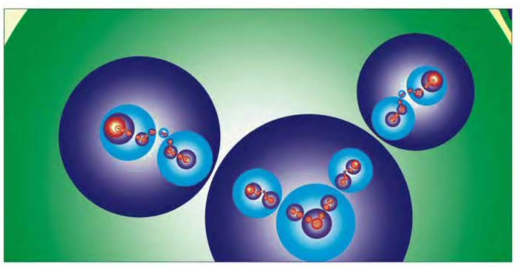
Now, if we do this with only one loxodromic Möbius transformation not much happens. If we apply \(a\) and \(A\) to these two circles multiple times we get smaller and smaller disks inside \(D_a\) and \(D_A\) that contain each one fixed point. Things get much more interesting if we take two loxodromic Möbius transformations \(a\) and \(b\) and their Schottky disks \(D_a\),\(D_A\),\(D_b\),\(D_B\). If we apply each transformation, so \(a\), \(A\), \(b\), \(B\), to each of the Schottky disks we get an image like this:
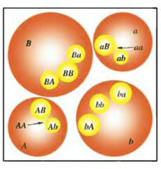
We call the image of \(D_A\) under the transformation \(B\) \(D_{BA}\), the image of \(D_A\) under \(D_b\) \(D_{bA}\) and so on. As you can see, on the second level we already have 12 Schottky disks. Now we apply each of the transformations to our 12 new Schottky disks we get this:
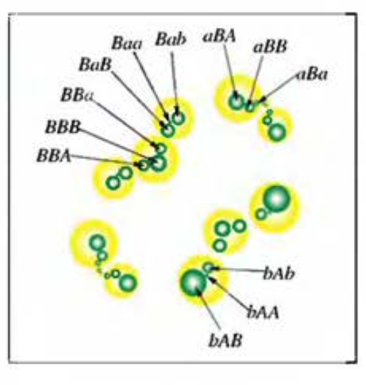
Now we apply our transformations to our 36 new Schottky disks and so on.
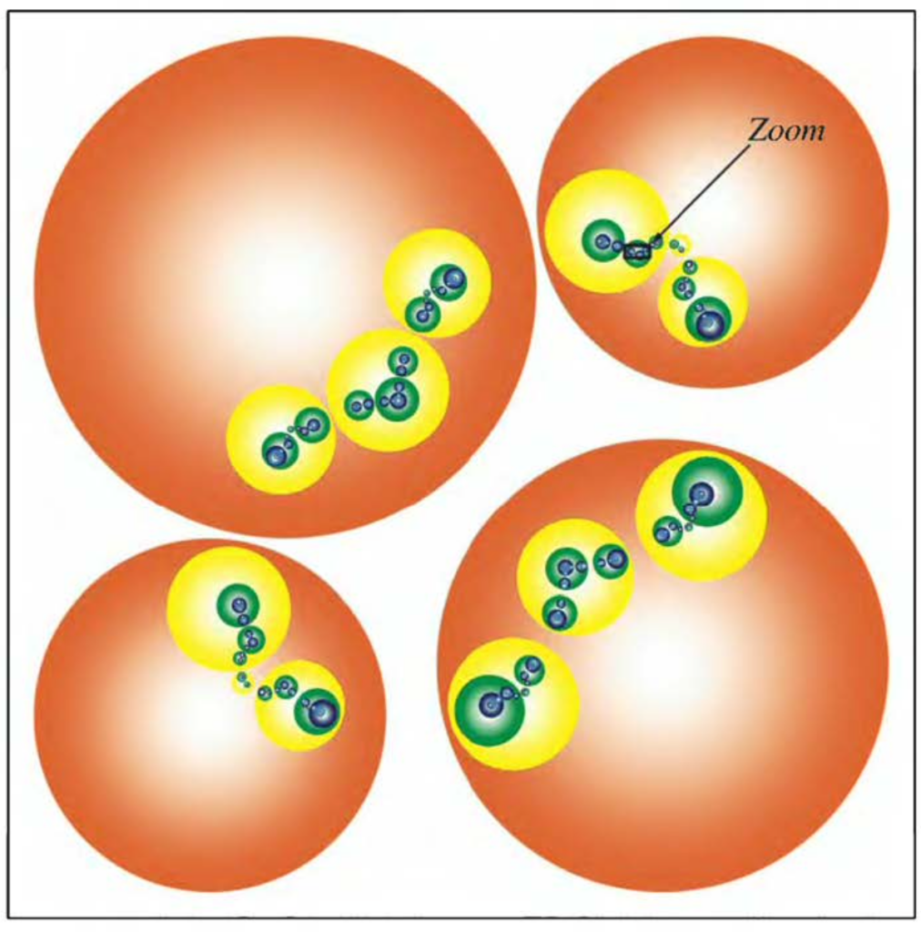
The book “Indras Pearls” [1] investigates the patterns that we get if we iterate this process.
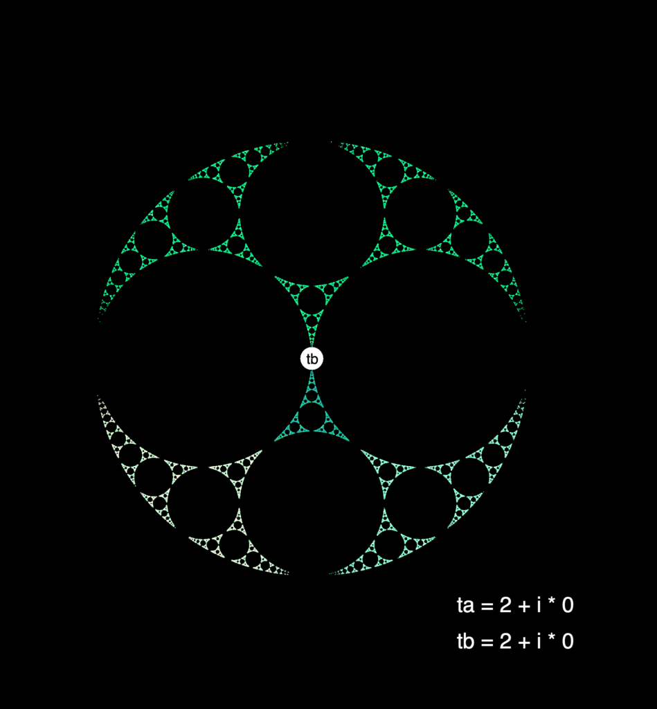
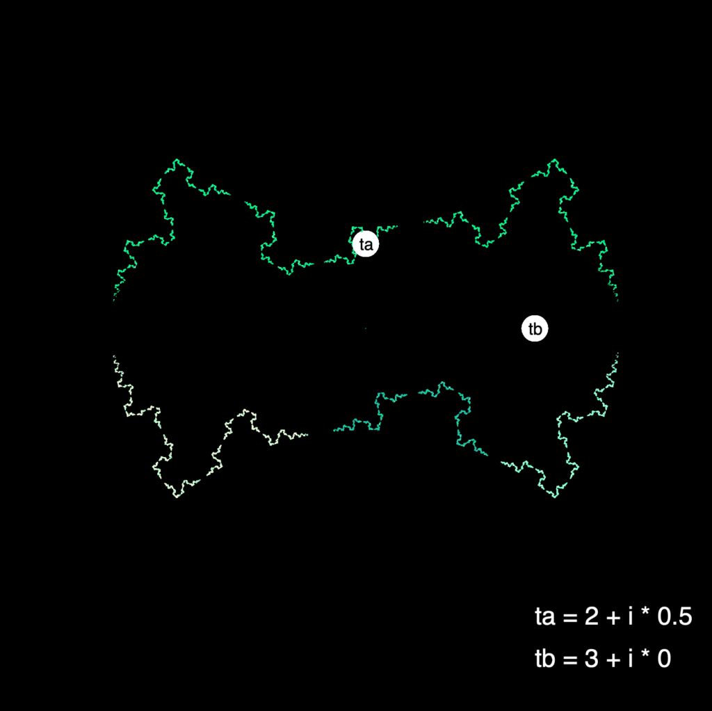
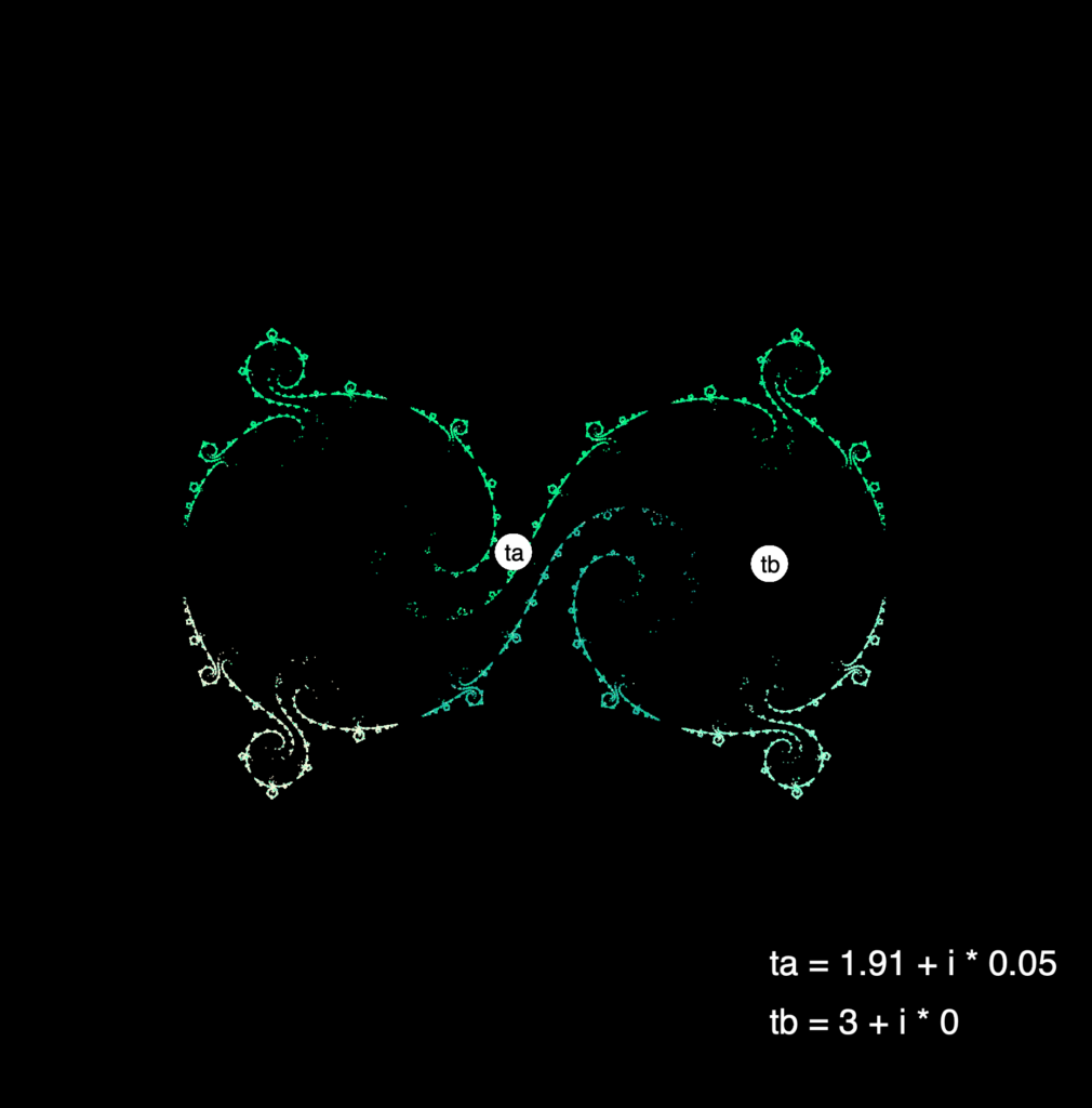
In each of these nesting circles, we can find a point that is going to be in every new circle, even if we do this process infinitely. We call the collection of points like this the limit set.
In the book, we find out that for some transformations \(a\) and \(b\) the limit set has a very interesting shape, e.g. a continuous, fractal shape.
The authors presented an algorithm they called “Grandmas Recipe” that gives us for two complex parameters \(t_a\) and \(t_b\) two transformations \(a\) and \(b\) where \(\text{trace}(a)=t_a\) and \(\text{trace}(b)=t_b\). The limit set generated by \(a\) and \(b\) is symmetrical under 180° rotation, and for many input parameters the limit set has a fractal shape.
Our program plots the limit set of these transformations we get from Grandmas recipe and lets you choose the input parameters by moving a slider in the complex plane or by typing it in manually.
We are using p5.js to plot the points that are supposed to represent our limit set.
The limit set consists of infinitely many points, so in reality it is pretty much impossible to plot the actual limit set by using points. Still, the book presents three algorithms that help us plot the limit set – or at least a very good approximation. For the first two, Breadth First Search and Depth First Search we chose a level, e.g. 500, and plot the according Schottky disks (they are going to be really small so we can take them as points). For an image that is a really good approximation to the limit set, we need a high level but since the number of points we would need to plot is equal to \(4\cdot 3^\text{lvl}\), these two methods are not suited for our interactive program. The method we are using is based on Barnsley’s Iterated Function System (IFS) method.
For the IFS method we use the fact that each loxodromic möbius transformations has two fixed points. We have already learned that successive powers of the transformation a shrink the disk \(D_a\) to the fixed point \(\text{Fix}^+(a)\), and the same goes for \(A\) with \(\text{Fix}^-(a)\) and vice versa for \(b\) and \(B\). Thus we know that the fixed points are in the limit set. So we choose our initial point or seed point \(z^{(0)}\) to be a fixed point of one of the generating matrices. Now what we do figuratively, is we let this point jump around in the limit set. We do this by applying a random generator to this point, so we get a sequence of points \(z^{(k)}\) defined by \(z^{(k+1)}=x^{(k)}(z^{(k)})\) where \(x^{(k)}\in\{a,A,b,B\}\) and is chosen randomly. If we plot these points, we get an image that pretty accurately approximates the limit set. Here are some pretty pictures that we got with our program:
References:
[1] Mumford, D., Series, C., & Wright, D. (2002). Indra’s Pearls: The Vision of Felix Klein. Cambridge: Cambridge University Press.