A comprehensive study on cooperation and cosponsoring in the US Senate
Written by Ayşegül Peközsoy, Leo Späth, and Klaus Stier
Political Background
The United States of America is a federal republic with a presidential system, meaning that the executive branch is dominated by the US president. The legislative branch is bicameral, i.e., there are two chambers (House of Representatives and Senate) which make up the US congress.
The 435 members of the House are elected for two years. In contrast, the members of the Senate are elected for six years. There are 100 senators, two of them represent one US state. Due to its voting system, almost all seats in congress are occupied by members of the two big political parties (Republican party and Democratic party). Thus, there is a well-established two-party system in US politics, since all parliamentarians belong to one of the two big parties mentioned above, with some few exceptions
In the following paper, we want to analyze cooperation between these parties. For our analysis, we focused on the Senate, since there is less fluctuation in its members. This is a very desirable feature, since cooperation is influenced by long-term bonds between individuals. In order to obtain a better understanding of cross-party cooperation, we mainly want to consider the legislative process, i.e., how bills are proposed and finally become law. Therefore, we want to outline the peculiarities of this process quickly.
In the Senate, each bill is introduced by one particular senator (called the sponsor of the bill). Other senators can work on the bill together with the sponsor and support the introduction of the bill, those senators are called cosponsors. As sponsor and cosponsors work together on the bill and its exact details, this relationship indicates at least some personal bond and connection between the actors involved. Apart from that, sponsor and cosponsors seem to share some political aims, since they agreed on introducing the bill together. Thus, cosponsorship indicates both personal and political closeness, what makes it a suitable measurement for cooperation between Republicans and Democrats.
After a bill has been introduced to the Senate, there are several readings and the bill is discussed. After that, the senators have to take a vote on the matter of the bill. If the Senate is in favor of the bill, it is passed on to the House of Representatives, as both chambers have to accept a bill in order for it to become law.
After this short introduction, let’s continue to focus on methodology.
Methodology
The main data used in our analysis was obtained from an API by the US government which provides information on bills in the legislative process. We decided to focus on analyzing the US Senate.
For our project, we took into account data from congress 93 (January 1973 – January 1975) until congress 117 (January 2021 until January 2023). For these congresses, detailed information on every bill that was introduced to the Senate is offered. In particular, the API also covers bills in this period that did not become law. However, since the main interest of our research was measuring and quantifying cross-party cooperation by looking at cosponsorship data, it seemed reasonable to use both bills that became law and bills that did not.
For earlier congresses however, only those bills were available that actually became law. In fact, only quite a small percentage of bills introduced are accepted by the Senate. Since the changes in the data base outlined above seem to be quite tremendous, we decided to not cover earlier periods. Covering those would have certainly led to a bias in our results.
Based on this data, we wanted to get a better idea of cross-party cooperation and cosponsorship and dynamics connected to these subjects. The following list contains a couple of questions that served as guiding questions for our research:
- How did cross-party cooperation change over time?
- Do policy areas differ in the extent to which cross-party cooperation takes place? What are policy areas with high/low rates of cross-party cosponsorship?
- What factors influence cooperation and cosponsorship?
- How can we group senators according to cosponsorship? What clusters can we identify?
The API provides all data that’s necessary to answer these questions (and a lot more). For instance, each bill has one particular policy area assigned to it (out of a list of 32 pre-defined areas), so questions that aim at cosponsorship in different political areas are feasible (the number of bills with no area assigned is negligibly small). In order to find answers to the issues above, different approaches were utilized.
Approach 1: Significant Cosponsoring Pairs
The main idea of this approach was to interpret the given data as a bidirected graph. The nodes of this graph are the senators, cosponsorings are edges between them. The graph is directed, since there is a difference between “getting cosponsored by someone” (receiving support) and “cosponsoring someone” (giving support). The graph is a weighted graph as well, as the number of cosponsorings per congress period are added to each edge as a weight.
However, this graph might be pretty confusing due to a high number of edges. To counter this, we want to remove noisy edges from the graph, i.e., remove cosponsoring pairs with low weights. After filtering those out, the significant cosponsorings remain. As these senators worked together quite often, it is quite likely that they indeed have some personal connection and have some political believes in common. In our context, we are particularly interested in significant cross-party cosponsorings, as they might give us a good impression of the state of cooperation between Republicans and Democrats.
The crucial point however is determining the threshold for deciding, whether a cosponsoring pair is significant or not. We came up with the following procedure for this:
- Determine the same-party pairs of cosponsoring and the cross-party pairs.
- Choose a quantile \(\alpha\) (such as 0.8 or 0.85). Compute the \(\alpha\) quantile of same-party pairs. We then have a threshold indicating the top pairs in same-party cooperation. Call these pairs \(SSP\) (significant same-party).
- Determine the cross-party pairs that have a number of cosponsorings that is higher or equal to the threshold computed in step 2. Call these pairs \(SCP\) (significant cross-party).
We want to quickly motivate and justify this procedure. In general, most senators might tend to work together with people from their own party (as people within a party share political aims, that’s why they are in the same party). If a cross-party pair has more cosponsorings than 80 or 85 percent of the same-party pairs, this clearly indicates that cooperation between these senators is based on (at least some) shared ideals and is not just a once in a blue moon thing.
Now we have the sets \(SSP\) and \(SCP\). With these sets, we can construct some simple measures for cross-party cooperation. For simplicity, use the following notation:
\(CP = \# SCP\)
\(SP = \# SSP\)
The first measure we construct gives us the share of \(SCP\) pairs out of all significant cosponsoring pairs (both \(SCP\) and \(SSP\)). We will also reference this measure as “\(CP\) by all”.
\( CP_\text{all} = \frac{CP}{CP + SP}\)
Moreover, one can also consider the number of significant cosponsoring pairs relative to the total number of bills in the Senate during that congress period (we denote the number of bills with \(N_b\)).
\( CP_\text{bills} = \frac{CP}{N_b} \)
Apart from constructing these measures and analyzing the sets \(SSP\) and \(SCP\) numerically, we also used a rather graphical method to get an impression of cooperation in the US Senate. For this purpose, we used the program Gephi. Gephi allows you to draw graphs and run e.g. clustering algorithms on them. Particularly when we have the senators grouped into 3 or 4 clusters, it is interesting to see whether mostly senators from the same party are grouped together, or whether we also obtain large “mixed” clusters. As one can see in the Results section, the visualizations with Gephi can be quite telling when it comes to cross-party cooperation.
Approach 2: Spectral Clustering
Spectral clustering is a very insightful tool to analyze social networks. However, it is a quite complex tool as well. Thus, we decided to dedicate an entire chapter to the spectral clustering approach and the results it yields.
Results
In this section, we want to give an overview about our results and findings. We start with a graph addressing the changes in the measure “\(CP\) by all” over the last 50 years. As can be seen easily by considering the construction of this measure in the previous section, higher values in this measure indicate a higher share of significant cross-party cosponsorings and thus more cross-party cooperation. There, we also constructed a measure \(CP_\text{bills}\). When plotting the values of this measure, we obtain a graph that is very similar to the graph for “\(CP\) by all”, so we only show the graph for “\(CP\) by all” to avoid repetition.
In the graph below, some further information has been added. On top, you can see the governing US president during the respective congress period. The time line below the graph is either marked green or red. Red indicates a divided Senate, i.e., the president’s party had no majority in the Senate during that period. Green, on the other hand, indicates that Oval Office and Senate majority belonged to the same party.
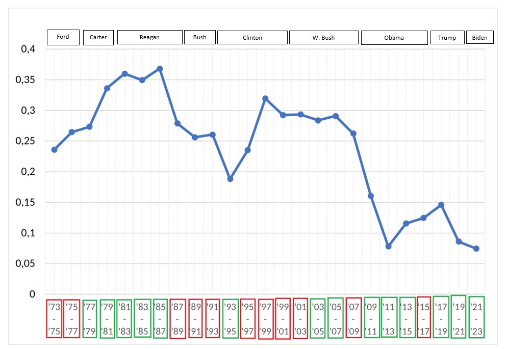
This chart shows that over the course of history, there have been ups and downs in the extent of cross-party cooperation. However, over the last ten years the cooperation rate seems to be eminently low. At the same time, one should take into account that during these period, the president’s party often had the senate majority as well, which reduces the necessity for cross-party cooperation.
Nevertheless, it’s worth mentioning that in earlier congress periods, there have been situations like these as well and they led to high numbers in cooperation, which contrasts the happenings of the last decade somewhat.
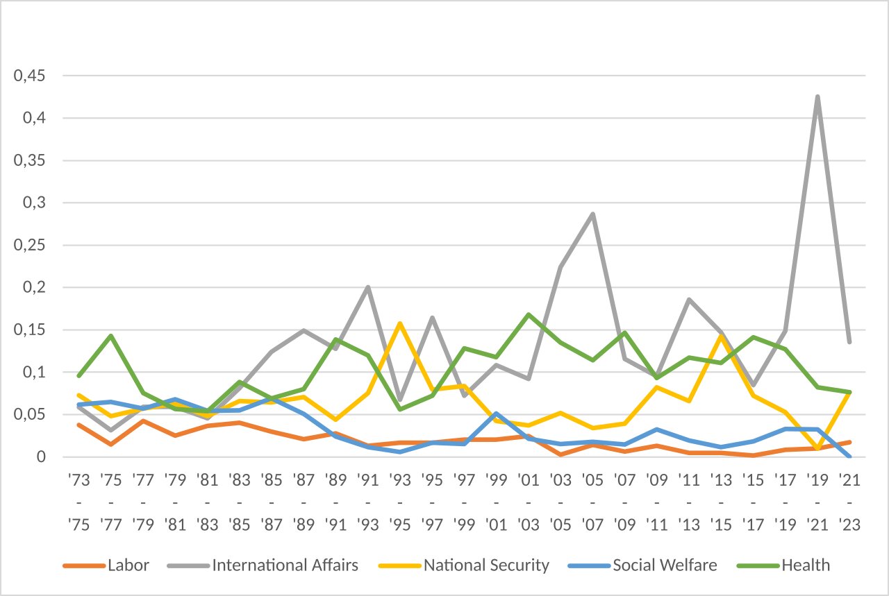
Moreover, it might be worth looking into what policy areas contributed most to cross-party cooperation. For analyzing this, we did the following: We took the \(SCP\) pairs and looked at the policy areas of the bills associated to each significant cross-party cosponsorship pair. Then we computed a percent-value for each policy area, telling how many significant cosponsorings are rooted in this particular area in the given congress period.
The graph below shows some of the results obtained from this inquiry. As we can see, there are areas that seem to have never been that suitable for cross-party cooperation, such as Labor or Social Welfare. On the other hand, one can see that e.g. International Affairs has some very high values during certain periods. That indicates that global happenings and international problems might require parties to work together and cooperate.
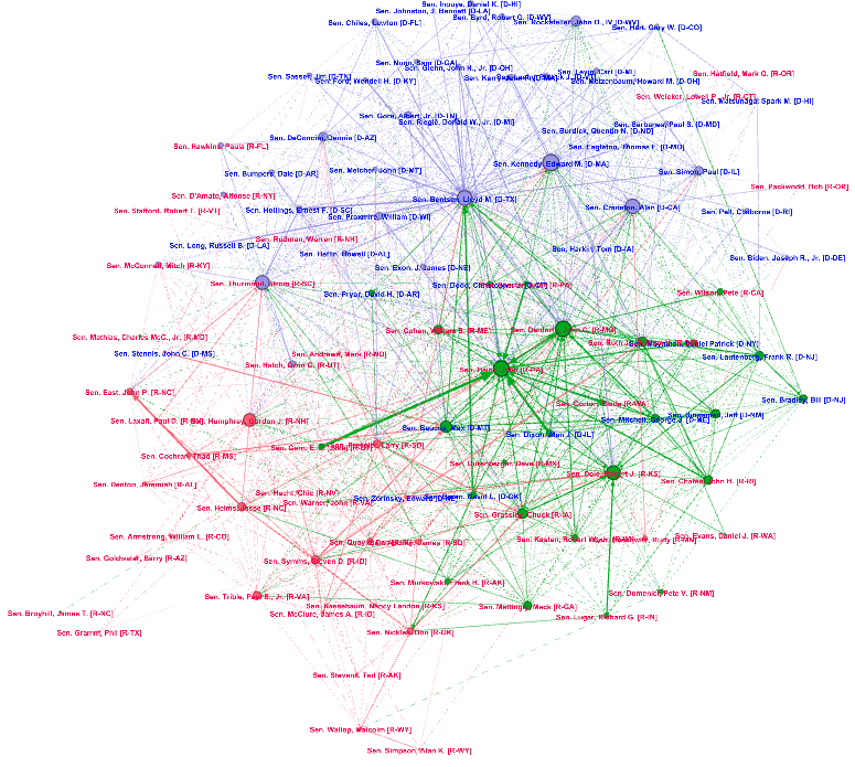
In addition to that, it is worthwhile to look at some graphs created with Gephi, as they convey a visual impression of whether we have a state of cooperation or separation in the US Senate. Moreover, one is able to recognize clusters and connected groups of senators. With this kind of visualization, it is also displayed whether a senator has a lot of cross-party cosponsorings and is an essential player for cross-party cooperation, or whether a senator is barely cooperating at all.
Before we present the graphs, some parts of the visualization should be explained briefly. As mentioned in the previous section, nodes represent senators and edges represent cosponsorings between individual senators. The graphs show both significant same-party cosponsoring and significant cross-party cosponsoring. The name of each senator is colored according to party affiliation (Republicans: red, Democrats: blue). The respective nodes, however, are colored according to which cluster they belong to. We ran clustering algorithms and tried to receive three or four clusters per graph to group the senators. Most of the time, we will get one cluster that is majorly Republican and one that will be majorly Democratic. We will color this clusters in the respective colors for simplicity. Nonetheless, there will also be Republican senators in the majorly Democratic cluster and vice versa. According to whether these clusters are strongly mixed or rather homogeneous, we might see a Senate based on either cooperation or separation.
Apart from the majority Republican and majority Democratic cluster, we also have some other (usually smaller) clusters, e.g. colored in green. As can be seen on the following graphs, these cluster usually consist of senators from both parties that have connections to both the majority Republican and the majority Democratic cluster. Thus, these smaller clusters (together with some other senators) stick the parties together.
One should also quickly pay attention to the edge thickness and the node thickness. Thick nodes and edges represent a high number of cosponsorings, whereas thin nodes and edges indicate fewer cosponsorings. With that being said, let’s have a look at some graphs.
The first graph (figure 3.3) deals with the Senate period from January 1985 until January 1987. As we can see, the Senate overall looks quite connected. From figure 3.1, we can tell that this was a Senate period with a comparably high extent of cosponsorings. This can be seen in the Gephi graph in several ways: First, we see that the green cluster (which connects the parties) is quite large. Moreover, we can find some Republican senators in the majority Democratic cluster and vice versa. There does not seem to be a sharp division line between the parties, cosponsoring happens in a cross-party fashion often. Thus, we can visually see that during this period cooperation between Republicans and Democrats worked well.
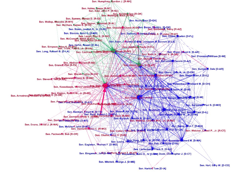
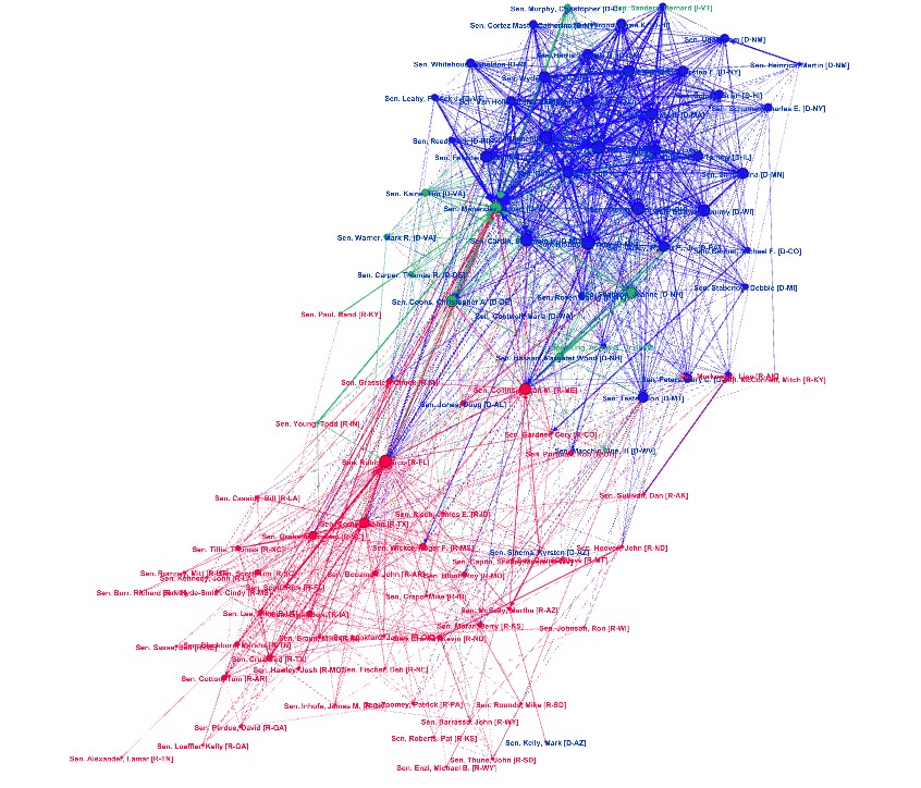
Figure 3.4 shows the Senate period from January 2019 until January 2021 and draws a somewhat different picture. The majority Democratic and the majority Republican cluster drifted apart spatially in the visualization, since there are not a lot of connections (i.e., cosponsorings) between them. Moreover, the green cluster is quite small and the separation line between the two parties seems to be sharp, as there are not a lot of Democratic senators in the majority Republican cluster (and vice versa). Hence, we can definitely say that during this Senate period, cross-party cooperation was considerably low. This perfectly fits into the observations from figure 3.1, as the respective period was one of the periods with the lowest rates of cosponsorings over the last 50 years.
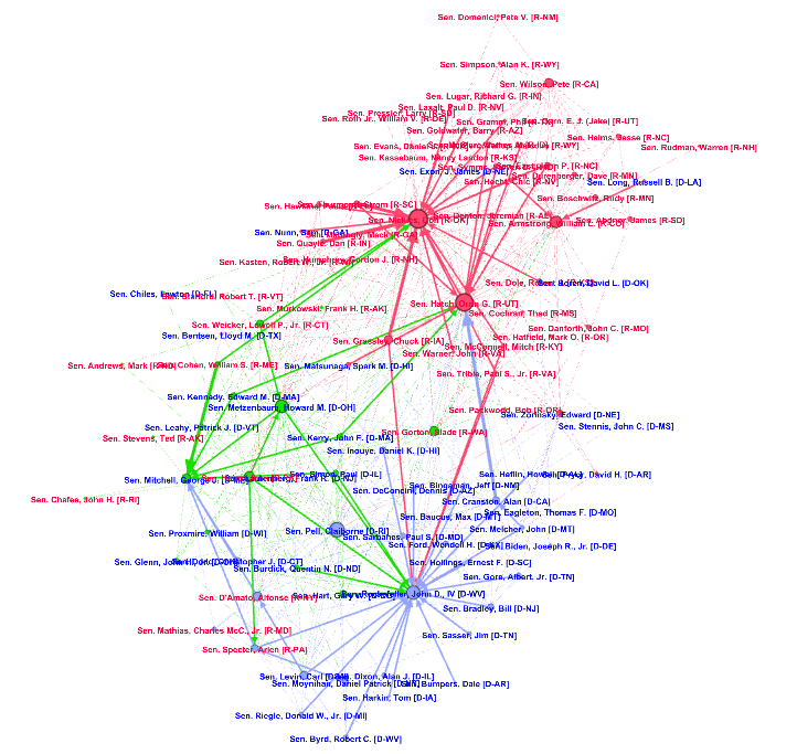
In addition to that, we can also use Gephi to visualize cosponsorship within a certain policy area and analyze distinct structures within particular areas. Let’s consider the Senate period from January 1985 until January 1987. In figure 3.3, we have seen that during this period, the Senate seemed quite connected. However, this picture might change according to which specific policy area is considered.
Figure 3.5 only considers cosponsorings concerning International Trade. In this graph, we still see a lot of cross-party cosponsorship, the two parties have cooperated on this area during that time considerably. In contrast to that, the graph in figure 3.6 does not look that connected anymore, most of the cosponsorings are within one party, there are only a few cross-party cosponsorings. This figure involves all cosponsorings from the area Labor and Employment, so we can notice a smaller degree of cross-party cooperation in this policy area.
Thus, we see that even though during this Senate period there has been a lot of cross-party cooperation, this does not necessarily mean that the same is true within every policy area during that time. Visually, we can see that there seems to be a considerable difference in the extent of cross-party cooperation when comparing International Trade and Labor and Employment.
Spectral Clustering Approach
Idea
In this section, our aim is to find a two-dimensional representation of the senators. Senators who have a higher number of mutual cosponsorings should be placed closer to each other.
\(n\ \text{Senators} \overset{\text{By number of cosponsorings}}{\longrightarrow}\ \text{Position} \ \hat{a}_i\ \text{for every Senator}\ i \)
We solve this problem by a method called Spectral Clustering. This approach provides a mathematically legitimate arrangement of the senators.
This can be used to graphically illustrate the cooperation of senators and factions based on cosponsorships of individual senators as well as Democrats and Republicans. Furthermore, we can calculate some measures that quantify the connectedness between the factions.
Mathemtical Aspects
Let \(W_{i,j}\) be the number of cosponsorings between the senators with numbers \(i\) and \(j\). Then the Spectral Clustering representation in the \(n\)-dimensional space is the collection of vectors \(\hat{a}_i\) for every senator \(i\) that minimize the value of:
\(\sum_{i,j} W_{i,j} \cdot { \vert \vert \hat{a}_i – \hat{a}_j \vert \vert }^{2}\)
under the normalization constraints:
(i): \(< \mathbb{D1} , a_{j} > = 0\)
(ii): \(< \mathbb{D} a_{j}, a_{j} > = n\)
for every \(j\) in \({1, … , n}\), where:
- \(a_{j}\) is the vector of the \(j\)-th components of all vectors \(\hat{a}_i\). (Note that \(\hat{a}_j\) is not the same as \(a_{j}\).)
- \(\mathbb{D}\) is the diagonal Matrix where the \(i\)-th entry on the diagonal is the number of cosponsorings of the \(i\)-th senator in total.
The idea of the formal approach is simple: If two senators have a high number of cosponsorships, the distance between their representing vectors should be as small as possible to minimize the term above.
We do not go into detail, but note the following:
- The minimization problem can be solved exactly as an (generalized) eigenvalue problem. For details, see the tutorial in [1].
- Compared to other methods of Multidimensional Scaling, this method not only considers the relationships between individual pairs of senators. Rather, the connections between several senators are also taken into account.
- The normaliziations constraints are important to exclude the trivial solutions:
\( \hat{a}_i = 0 \quad \text{for every}\ i \)
and the possibility to get step-by-step better solutions \(\hat{a}_i’\) from \(\hat{a}_i\) by the iteration:
\( \hat{a}_i’ \leftarrow \frac{1}{2} \cdot \hat{a}_i \) - The spectral clustering method is only useful in cases where we have a huge amount of connectedness between the senators. If there are groups without any connection, it does not work very well.
Party Analysis
For our further analyisis, we use only the first two components of the vectors \(a_{i}\) which represent the senators to avoid the “curse of dimensionality”.
From this, we calculate different measures that measure the difference between the Democrats and the Repuclicans. We do the analysis for the 117th congress, where we group the two independent senators Angus King and Bernie Sanders to the Democrats, like they belong to this faction in the Senate. The measures we calculate are:
\(\text{Measure1} = \frac{\text{AverageEucDistanceDemocrats} + \text{AverageEucDistanceRepuclicans} }{\text{AverageDistanceAllSenators}}\)
\(\text{Measure2} = \frac{\text{AverageEucDistanceDemocrats}^{2}+ \text{AverageEucDistanceRepuclicans}^{2} }{\text{AverageDistanceAllSenators}^{2}}\)
\(\text{Measure3} = \frac{\text{eucDistance}(\text{centerReps},\, \text{centerDems})}{\sqrt{\text{varAllSenators}}}\)
\(\text{Measure1}\) calculates the ratio between the sum of the average euclidean distance within the two factions and the average euclidean distance of all senators. \(\text{Measure2}\) does the same, but it uses the squared values of the averages.
For \(\text{Measure3}\) we look not only on unique senators, but also on the the whole factions. So we calculate the distance between the centers of the cluster of the senators belonging to the Democrats and the senators belonging to the Repuclicans. For a better comparability, we normalize this number by dividing it by the (empirical) standard deviation of all senators (interpreted as representations of random variables).
A higher number of cosponsorings between senators from different factions results in a lower value of the denominator of \(\text{Measure1}\) and \(\text{Measure2}\). Because of this, \(\text{Measure1}\) and \(\text{Measure2}\) increase in this case.
On the other site, a higher number of cosponsorings between senators from different factions results in a lower value of the nominator of \(\text{Measure3}\). Because of this, \(\text{Measure3}\) decreases in this case.
Results
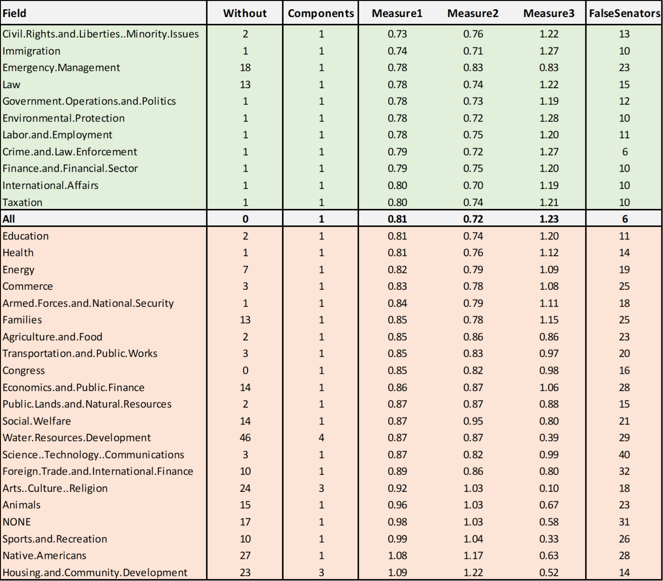
For the 117th Senate, we calculate the following values for each of the 32 political fields,
the collection of the bills that are not connected to a field and the collection of all bills:
- Without: The number of senators who have no cosponsoring.
- Components: The number of connected components of the senator-cosponsoring graph
(where to senators are connected if they have minimum one cosponsoring together.) - \(\text{Measure1}\), \(\text{Measure2}\), \(\text{Measure3}\) explained above.
- FalseSenators: The number of senators that have more cosponsorings with senators
from the other faction than with their own faction.
Discussion
The political fields with the lowest values of \(\text{Measure1}\) are Civil.Rights.and.Liberties..Minority.Issues and Immigration. The political fields with the highest values of \(\text{Measure1}\) are Native.Americans and Housing.and.Community.Development. The fields with the lowest values of \(\text{Measure2}\) are International.Affairs and Immigration. The fields with the highest values of \(\text{Measure2}\) are same as in \(\text{Measure1}\). All in all, the strength of collaboration between Democrats and Republicans in individual policy areas classified by measures corresponds to intuitive expectations.
Graphical Illustrations
The following graphics illustrate, by way of example, the vectors representing the senators found by the spectral clustering method (first two components). In our case, we limit ourselves to the fields CivilRightsandLibertiesMinorityIssues, Immigration, NativeAmericans, SportsandRecreation and the collection of the bills of all fields. In the graphics, a red dot resprents a senator from the Republicans, a blue dot a senator from the Democrats and an azure dot one of the two independent senators. In the caption of the graphics we note the values of \(\text{Measure1}\), \(\text{Measure1}\), and \(\text{Measure3}\) (M1, M2, M3) for the interesting fields.
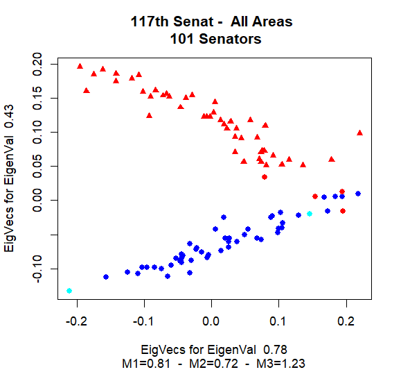
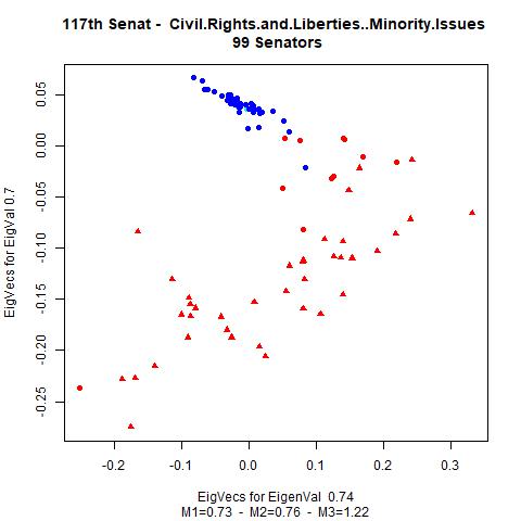
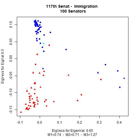
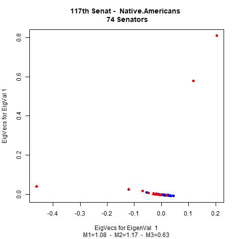
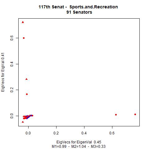
We see that the graphical illustrations correspondents to the mathematical results of the analysis.
Conclusion and Outlook
Overall, we can notice a significantly low rate of cooperation in the US Senate within the past ten years. However, one has to keep in mind the effects that ownership of both Oval Office and Senate majority by a single party might have on this. Apart from that, it was apparent that cross-party cooperation differs in distinct policy areas. While we might expect cooperation in areas such as International Affairs, this cooperation does not seem to take place in policy areas like Social Welfare or Labor.
There are several ways in which one could deepen this analysis. For now, we only have been looking at party affiliation. However, it might be worthwhile to take into consideration other characteristics of senators (such as e.g. the state one represents or the degree of political experience) and analyze the impact these factors have in cross-party cooperation.
Furthermore, one could consider other peculiarities of the legislative process to obtain insights about the state of cross-party cooperation. Instead of looking at cosponsorship, we could take into account how often certain parliamentarians had a similar behaviour in ballots for bills (for the House of Representatives, this is done in [2]).
Apart from that, the code we wrote would also allow to track cosponsorship down to a personal level. One could analyze how cosponsorship relations of a single senator changed over time. This seems particularly promising, as senators are elected for six years and most of them are re-elected a couple of times, so some of them end up serving for decades. It would be interesting to see whether large-scale changes that have been detected in this analysis can be seen on a personal level in the same way and extent.
References:
- Ulrike von Luxburg, 2007. A Tutorial on Spectral Clustering. In Statistics and Computing, 17 (4), 2007.
- Clio Andris et al., 2015. The Rise of Partisanship and Super-Cooperators in the U.S. House of Representatives. In PLoS ONE, 10 (4), 2015.